User Guide#
This notebook walks through how to use the Datawaza functions for data exploration, cleaning and modeling. It doesn’t cover everything you need to do in a typical project. It just shows how you might incorporate the Datawaza functions into your existing workflow.
Table of Contents#
-
Get Unique Values - get_unique()
Plot Charts - plot_charts()
Get Outliers - get_outliers()
Get Correlations - get_corr()
Plot Correlations - plot_corr()
Plot 3D Chart - plot_3d()
Plot Map of California - plot_map_ca()
Plot Scatterplot - plot_scatt()
Print ASCII Image - print_ascii_image()
-
Convert Data Types - convert_dtypes()
Convert Data Values - convert_data_values()
Convert Time Values - convert_time_values()
Split Outliers - split_outliers()
Reduce Multicollinearity - reduce_multicollinearity()
-
Create Pipeline - create_pipeline()
Iterate Model - iterate_model()
Create Results DataFrame - create_results_df()
Run Multiple Iterations - iterate_model()
Plot the Results - plot_results()
Plot ACF Residuals - plot_acf_residuals()
Evaluate Classification Model - eval_model()
Compare Models - compare_models()
Compare Binary Classification Models - compare_models()
Plot the Best Models - plot_results()
Compare Multi-Class Classification Models - compare_models()
Create Binary Classification Neural Network - create_nn_binary
Create Multi-Class Classification Neural Network - create_nn_multi()
Plot Training History - plot_train_history()
-
Log Transform - log_transform()
Check for Duplicates - check_for_duplicates()
Split Dataframe - split_dataframe()
Format Dataframe - format_df()
Format Chart Axis as Dollars - dollars()
Format Chart Axis as Thousands - thousands()
Calculate VIF - calc_vif()
Calculate PFI - calc_pfi()
Extract Coefficients - extract_coef()
Getting Started#
Install Datawaza#
Install Datawaza with pip:
pip install datawaza
Because Datawaza’s functions cover a broad set of use cases, it requires a number of packages to be installed. But most of these should already be in your environment if you’re doing Data Science or Machine Learning.
Import Libraries#
You can import the entire library as follows:
import datawaza as dw
Alternatively, you can import select modules. For instance, if you only want to use the model pipeline and iteration tools:
from datawaza import model
In this guide, we’ll import the complete Datawaza library and use the dw prefix before any of it’s functions:
[1]:
# Data processing libraries
import numpy as np
import pandas as pd
# Charting libraries
import matplotlib.pyplot as plt
import seaborn as sns
import plotly.express as px
from matplotlib.ticker import FuncFormatter
# Modeling workflow
from sklearn.pipeline import Pipeline
from sklearn.model_selection import train_test_split, KFold, StratifiedKFold
from sklearn.impute import SimpleImputer, KNNImputer
from sklearn.preprocessing import (OneHotEncoder, OrdinalEncoder, PolynomialFeatures, StandardScaler,
MinMaxScaler, RobustScaler, FunctionTransformer)
from sklearn.feature_selection import RFE, SequentialFeatureSelector
# Models used in some examples
from sklearn.linear_model import LinearRegression, LogisticRegression, Ridge
from sklearn.neighbors import KNeighborsClassifier
from sklearn.svm import SVC
from sklearn.tree import DecisionTreeClassifier, DecisionTreeRegressor
from sklearn.ensemble import RandomForestClassifier
from xgboost import XGBClassifier
from statsmodels.tsa.seasonal import STL
# Sample datasets
from sklearn.datasets import load_iris, load_wine, load_breast_cancer, make_classification
# Set environment flag to avoid TensorFlow warning
import os
os.environ['TF_CPP_MIN_LOG_LEVEL'] = '2'
# Import TensorFlow and Keras
from keras.callbacks import EarlyStopping
from scikeras.wrappers import KerasClassifier
from keras.utils import to_categorical
from keras.models import Sequential
from keras.layers import Input, Dense
# Import PyTorch
import torch
# Import Datawaza
import datawaza as dw
from datawaza.tools import LogTransformer
Explore#
The dw.explore module provides tools to streamline exploratory data analysis. It contains functions to find unique values, plot distributions, detect outliers, extract the top correlations, and plot correlations.
Get Unique Values - get_unique()
Plot Charts - plot_charts()
Get Outliers - get_outliers()
Get Correlations - get_corr()
Plot Correlations - plot_corr()
Plot 3D Chart - plot_3d()
Plot Map of California - plot_map_ca()
Plot Scatterplot - plot_scatt()
Print ASCII Image - print_ascii_image()
Load Data#
Let’s load some initial data and set some display preferences.
[2]:
# Read in the data in CSV format
df = pd.read_csv('data/bank-additional-full.csv', sep=';')
[3]:
# Set some display preferences
pd.set_option('display.max_columns', None)
pd.set_option('display.max_colwidth', None)
[4]:
# Show the first few records of data
df.head()
[4]:
| age | job | marital | education | default | housing | loan | contact | month | day_of_week | duration | campaign | pdays | previous | poutcome | emp.var.rate | cons.price.idx | cons.conf.idx | euribor3m | nr.employed | y | |
|---|---|---|---|---|---|---|---|---|---|---|---|---|---|---|---|---|---|---|---|---|---|
| 0 | 56 | housemaid | married | basic.4y | no | no | no | telephone | may | mon | 261 | 1 | 999 | 0 | nonexistent | 1.1 | 93.994 | -36.4 | 4.857 | 5191.0 | no |
| 1 | 57 | services | married | high.school | unknown | no | no | telephone | may | mon | 149 | 1 | 999 | 0 | nonexistent | 1.1 | 93.994 | -36.4 | 4.857 | 5191.0 | no |
| 2 | 37 | services | married | high.school | no | yes | no | telephone | may | mon | 226 | 1 | 999 | 0 | nonexistent | 1.1 | 93.994 | -36.4 | 4.857 | 5191.0 | no |
| 3 | 40 | admin. | married | basic.6y | no | no | no | telephone | may | mon | 151 | 1 | 999 | 0 | nonexistent | 1.1 | 93.994 | -36.4 | 4.857 | 5191.0 | no |
| 4 | 56 | services | married | high.school | no | no | yes | telephone | may | mon | 307 | 1 | 999 | 0 | nonexistent | 1.1 | 93.994 | -36.4 | 4.857 | 5191.0 | no |
[5]:
# Examine the data types and null counts
df.info()
<class 'pandas.core.frame.DataFrame'>
RangeIndex: 41188 entries, 0 to 41187
Data columns (total 21 columns):
# Column Non-Null Count Dtype
--- ------ -------------- -----
0 age 41188 non-null int64
1 job 41188 non-null object
2 marital 41188 non-null object
3 education 41188 non-null object
4 default 41188 non-null object
5 housing 41188 non-null object
6 loan 41188 non-null object
7 contact 41188 non-null object
8 month 41188 non-null object
9 day_of_week 41188 non-null object
10 duration 41188 non-null int64
11 campaign 41188 non-null int64
12 pdays 41188 non-null int64
13 previous 41188 non-null int64
14 poutcome 41188 non-null object
15 emp.var.rate 41188 non-null float64
16 cons.price.idx 41188 non-null float64
17 cons.conf.idx 41188 non-null float64
18 euribor3m 41188 non-null float64
19 nr.employed 41188 non-null float64
20 y 41188 non-null object
dtypes: float64(5), int64(5), object(11)
memory usage: 6.6+ MB
[6]:
# Create some column lists we can use to target the right kind of variables
all_columns = list(df.columns)
num_columns = [col for col in all_columns if df[col].dtype in ['int64', 'float64']]
cat_columns = [col for col in all_columns if df[col].dtype in ['object', 'category', 'string']]
Get Unique Values#
dw.get_unique() prints the unique values of all variables below a threshold n, including counts and percentages.
This function examines the unique values of all the variables in a DataFrame. If the number is below a threshold n, it will list their unique values. For each value, it prints out the count and percentage of the dataset with that value. You can change the sort, and there are options to strip single quotes from the variable names, or exclude NaN values. You can optionally show descriptive statistics for the continuous variables able the n threshold, or display simple plots.
Use this to quickly examine the features of your dataset at the beginning of exploratory data analysis. Use df.nunique() to first determine how many unique values each variable has, and identify a number that likely separates the categorical from continuous numeric variables. Then run get_unique using that number as n (this avoids iterating over continuous data).
[7]:
# Look at unique value counts to choose an 'n' threshold between categorical and continuous
df.nunique().sort_values(ascending=False)
[7]:
duration 1544
euribor3m 316
age 78
campaign 42
pdays 27
cons.conf.idx 26
cons.price.idx 26
job 12
nr.employed 11
month 10
emp.var.rate 10
previous 8
education 8
day_of_week 5
marital 4
default 3
poutcome 3
loan 3
housing 3
contact 2
y 2
dtype: int64
[8]:
# Show the unique values of each variable below the threshold of n = 12
dw.get_unique(df, 12, count=True, percent=True)
CATEGORICAL: Variables with unique values equal to or below: 12
job has 12 unique values:
admin. 10422 25.3%
blue-collar 9254 22.47%
technician 6743 16.37%
services 3969 9.64%
management 2924 7.1%
retired 1720 4.18%
entrepreneur 1456 3.54%
self-employed 1421 3.45%
housemaid 1060 2.57%
unemployed 1014 2.46%
student 875 2.12%
unknown 330 0.8%
marital has 4 unique values:
married 24928 60.52%
single 11568 28.09%
divorced 4612 11.2%
unknown 80 0.19%
education has 8 unique values:
university.degree 12168 29.54%
high.school 9515 23.1%
basic.9y 6045 14.68%
professional.course 5243 12.73%
basic.4y 4176 10.14%
basic.6y 2292 5.56%
unknown 1731 4.2%
illiterate 18 0.04%
default has 3 unique values:
no 32588 79.12%
unknown 8597 20.87%
yes 3 0.01%
housing has 3 unique values:
yes 21576 52.38%
no 18622 45.21%
unknown 990 2.4%
loan has 3 unique values:
no 33950 82.43%
yes 6248 15.17%
unknown 990 2.4%
contact has 2 unique values:
cellular 26144 63.47%
telephone 15044 36.53%
month has 10 unique values:
may 13769 33.43%
jul 7174 17.42%
aug 6178 15.0%
jun 5318 12.91%
nov 4101 9.96%
apr 2632 6.39%
oct 718 1.74%
sep 570 1.38%
mar 546 1.33%
dec 182 0.44%
day_of_week has 5 unique values:
thu 8623 20.94%
mon 8514 20.67%
wed 8134 19.75%
tue 8090 19.64%
fri 7827 19.0%
previous has 8 unique values:
0 35563 86.34%
1 4561 11.07%
2 754 1.83%
3 216 0.52%
4 70 0.17%
5 18 0.04%
6 5 0.01%
7 1 0.0%
poutcome has 3 unique values:
nonexistent 35563 86.34%
failure 4252 10.32%
success 1373 3.33%
emp.var.rate has 10 unique values:
1.4 16234 39.41%
-1.8 9184 22.3%
1.1 7763 18.85%
-0.1 3683 8.94%
-2.9 1663 4.04%
-3.4 1071 2.6%
-1.7 773 1.88%
-1.1 635 1.54%
-3.0 172 0.42%
-0.2 10 0.02%
nr.employed has 11 unique values:
5228.1 16234 39.41%
5099.1 8534 20.72%
5191.0 7763 18.85%
5195.8 3683 8.94%
5076.2 1663 4.04%
5017.5 1071 2.6%
4991.6 773 1.88%
5008.7 650 1.58%
4963.6 635 1.54%
5023.5 172 0.42%
5176.3 10 0.02%
y has 2 unique values:
no 36548 88.73%
yes 4640 11.27%
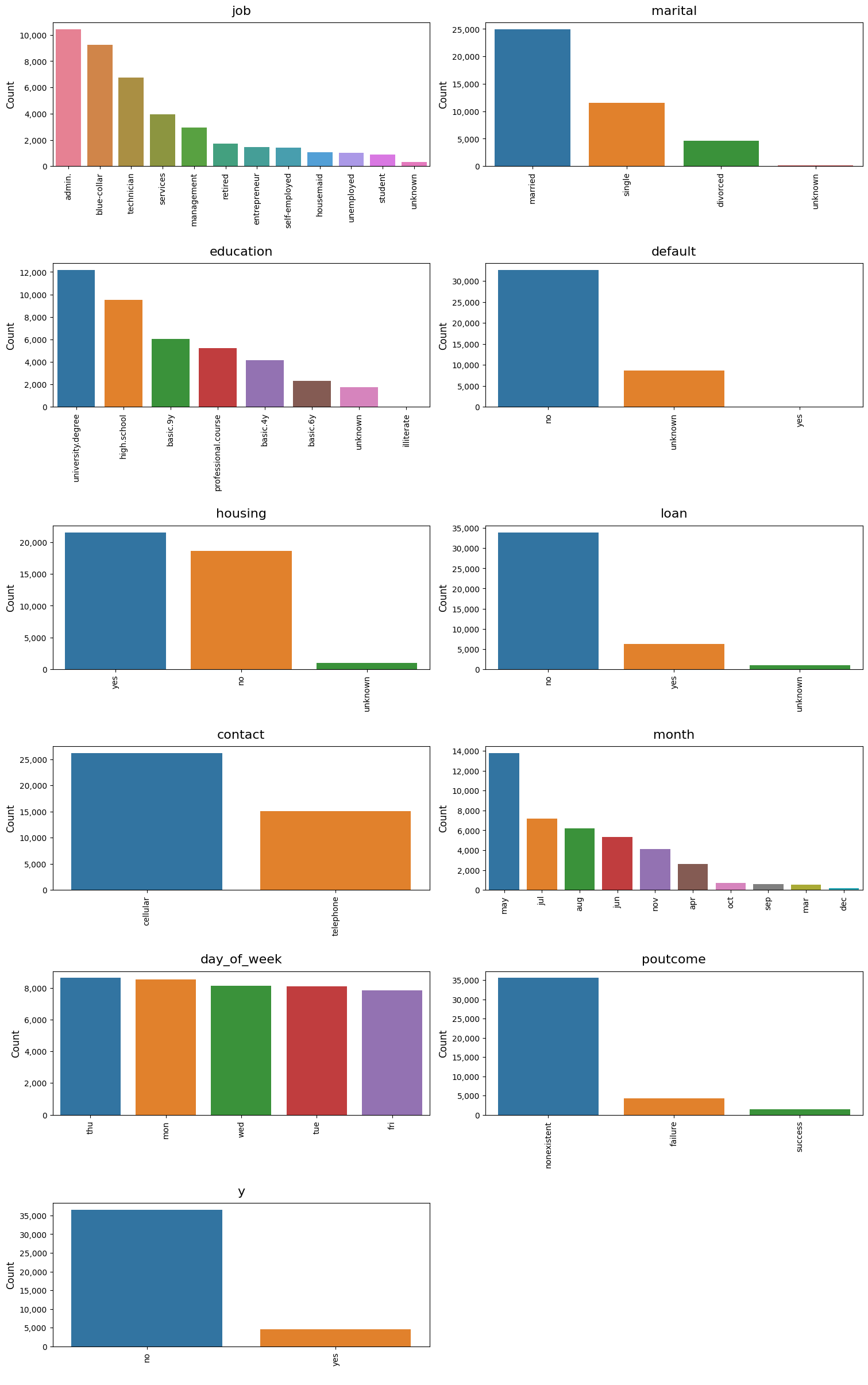
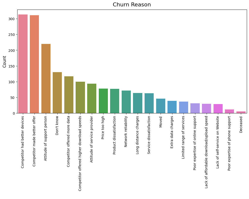
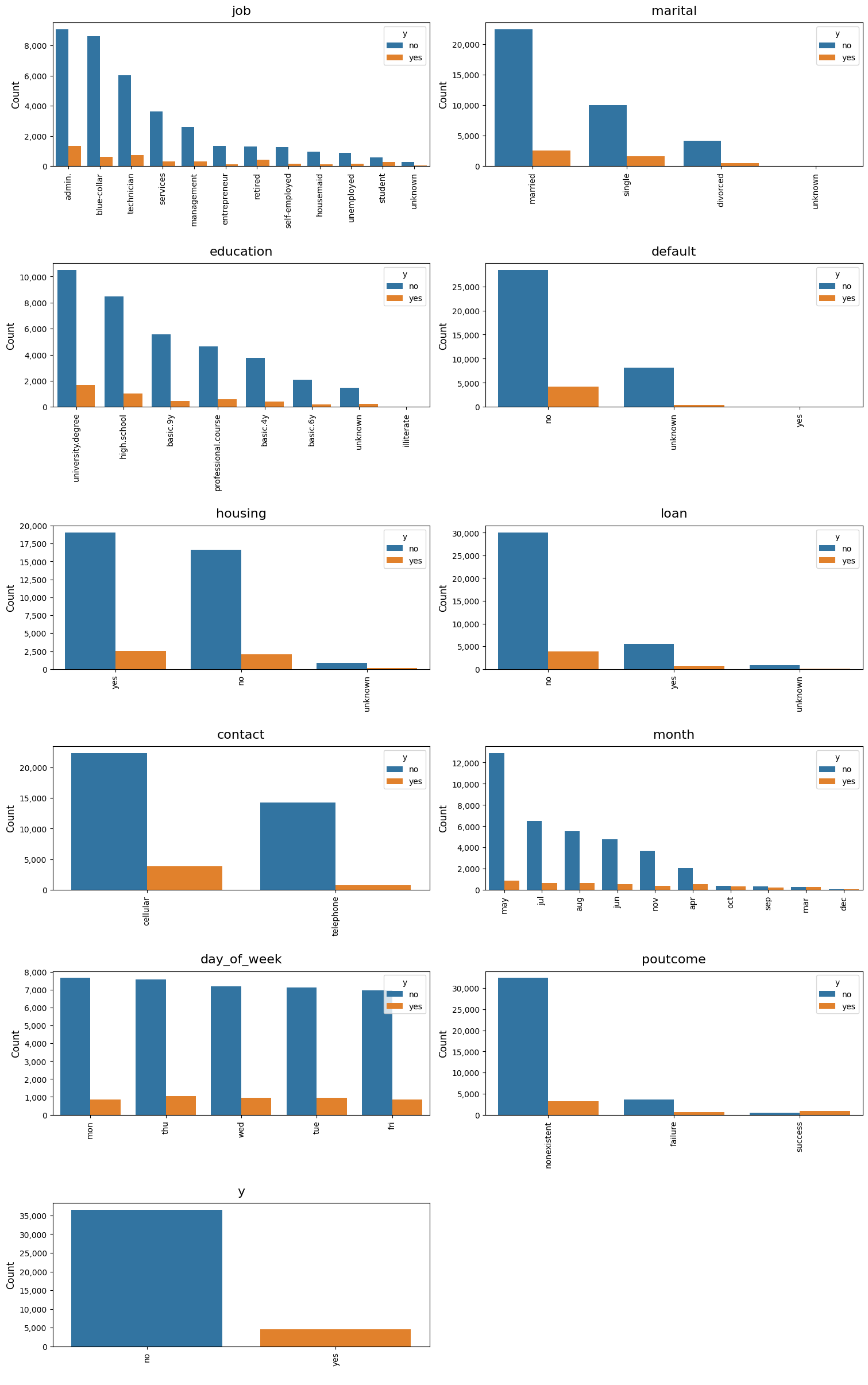
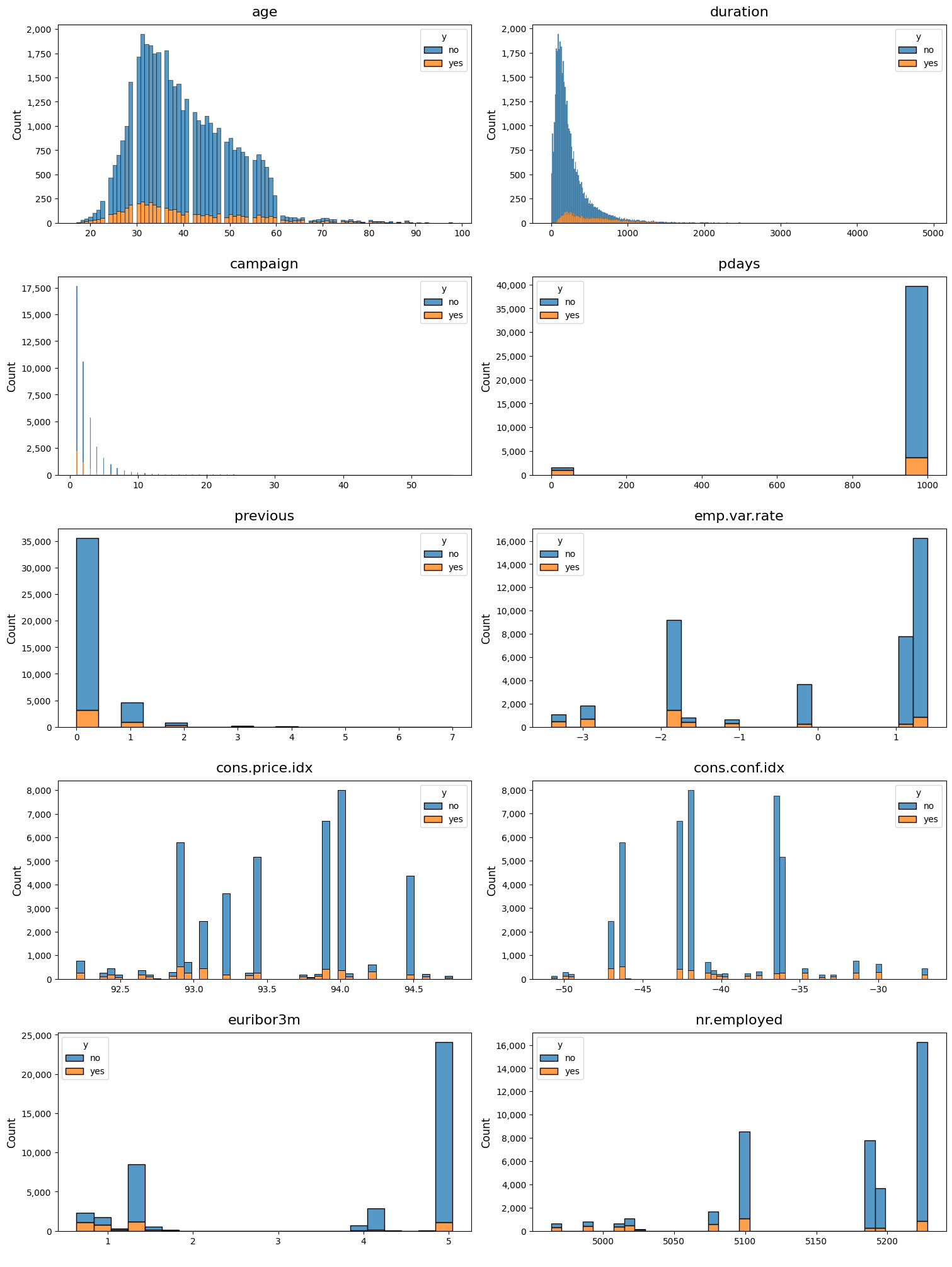
Plot Charts#
dw.plot_charts displays multiple bar plots and histograms for categorical and/or continuous variables in a DataFrame, with an option to dimension by the specified hue.
This function allows you to plot a large number of distributions with one line of code. You choose which type of plots to create by setting plot_type to cat, cont, or both. Categorical variables are plotted with sns.countplot ordered by descending value counts for a clean appearance. Continuous variables are plotted with sns.histplot. There are two approaches to identifying categorical vs. continuous variables: (a) you can specify cat_cols and cont_cols as lists
of the respective column names, or (b) you can specify n as the dividing line, and any variable with n or lower unique values will be treated as categorical. In addition, you can enable dtype_check on the continuous columns to only include columns of data type int64 or float64.
For each type of variable, it creates a subplot layout that has ncols columns, and is fig_width wide. It calculates how many rows are required to display all the plots, and each row is subplot_height high. Specify hue if you want to dimension the plots by another variable. You can set color_discrete_map to a color mapping dictionary for the values of the hue variable. You can also customize some parameters of the plots, such as rotation of the X axis tick labels. For
categorical variables, you can normalize the plots to show proportions instead of counts by setting normalize to True.
For histograms, you can display KDE lines with kde, and change how the hue variable appears by setting multiple. If you have a large amount of data that is taking too long to process, you can take a random sample of your data by setting sample_size to either a count or proportion. To handle skewed data, you have two options: (a) you can enable log scale on the X axis with log_scale, and (b) you can ignore zero values with ignore_zero (these can sometimes dominate the left
end of a chart).
Use this function to quickly visualize the distributions of your data during exploratory data analysis. With one line, you can produce a comprehensive series of plots that can help you spot issues that will require handling during data cleaning. By setting hue to your target y variable, you might be able to catch glimpses of potential correlations or relationships.
Categorical Distributions#
[9]:
# Plot bar charts of categorical variables
dw.plot_charts(df, plot_type='cat', cat_cols=cat_columns, rotation=90)
[10]:
# Load another dataset with a column that has a large number of categorical values
df_telco = pd.read_csv('data/df_telco.csv', index_col=0)
[11]:
# Plot a single chart for the larger value sets
dw.plot_charts(df_telco, plot_type='cat', n=25, cat_cols=['Churn Reason'], ncols=1, fig_width=10, subplot_height=8, rotation=90)
[12]:
# Plot bar charts of categorical variables, dimensioned by the target variable
dw.plot_charts(df, plot_type='cat', cat_cols=cat_columns, hue='y', rotation=90)
Continuous Distributions#
[13]:
# Plot histograms of continuous variables, dimensioned by the target variable
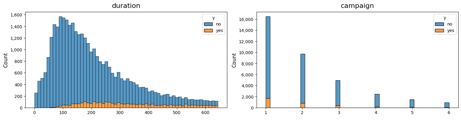
dw.plot_charts(df, plot_type='cont', cont_cols=num_columns, hue='y', multiple='stack')
Get Outliers#
dw.get_outliers() detects and summarizes outliers for the specified numeric columns in a DataFrame, based on an IQR ratio.
This function identifies outliers using Tukey’s method, where outliers are considered to be those data points that fall below Q1 - ratio * IQR or above Q3 + ratio * IQR. You can exclude zeros from the calculations, as they can appear as outliers and skew your results. You can also change the default IQR ratio of 1.5. If outliers are found, they will be summarized in the returned DataFrame. In addition, the distributions of the variables with outliers can be plotted as boxplots.
Use this function to identify outliers during the early stages of exploratory data analysis. With one line, you can see: total non-null, total zero values, zero percent, outlier count, outlier percent, skewness, and kurtosis. You can also visually spot outliers outside of the whiskers in the boxplots. Then you can decide how you want to handle the outliers (ex: log transform, drop, etc.)
[14]:
# Identify outliers, store in dataframe, and plot boxplots
outliers_df = dw.get_outliers(df, num_columns, plot=True, width=15, height=1)
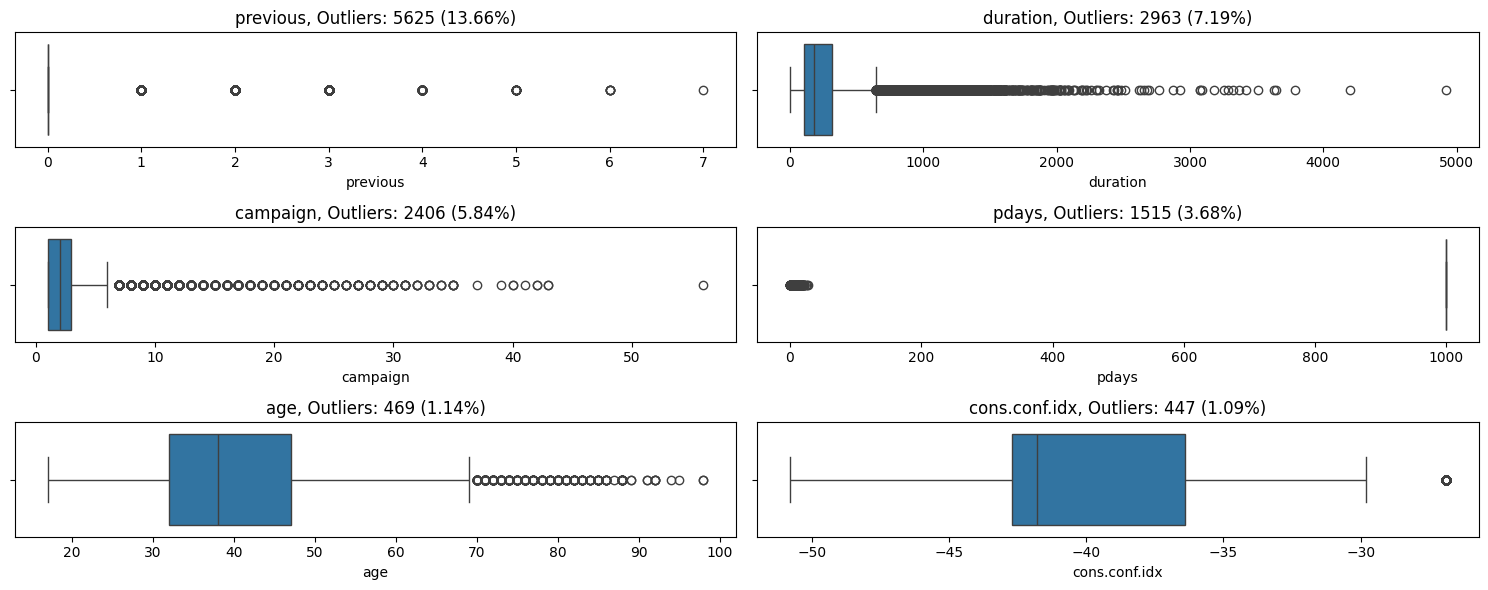
[15]:
# Display the dataframe with the output from detect_outliers
outliers_df
[15]:
| Column | Total Non-Null | Total Zero | Zero Percent | Outlier Count | Outlier Percent | Skewness | Kurtosis | |
|---|---|---|---|---|---|---|---|---|
| 4 | previous | 41188 | 35563 | 86.34 | 5625 | 13.66 | 3.83 | 20.11 |
| 1 | duration | 41188 | 4 | 0.01 | 2963 | 7.19 | 3.26 | 20.25 |
| 2 | campaign | 41188 | 0 | 0.00 | 2406 | 5.84 | 4.76 | 36.98 |
| 3 | pdays | 41188 | 15 | 0.04 | 1515 | 3.68 | -4.92 | 22.23 |
| 0 | age | 41188 | 0 | 0.00 | 469 | 1.14 | 0.78 | 0.79 |
| 5 | cons.conf.idx | 41188 | 0 | 0.00 | 447 | 1.09 | 0.30 | -0.36 |
[16]:
# Store the outlier columns in a list for easy reference
outlier_columns = list(outliers_df['Column'])
[17]:
# Show the outlier column list values
outlier_columns
[17]:
['previous', 'duration', 'campaign', 'pdays', 'age', 'cons.conf.idx']
Load Encoded Data#
Let’s now load some encoded data, where everything is numeric, so we can demonstrate the correlation functions.
[18]:
# Load a previously cleaned and encoded dataset (processing not shown here)
df_enc = pd.read_csv('data/df_enc.csv')
df_enc.drop(['subscribed'], axis=1, inplace=True)
[19]:
df_enc.head()
[19]:
| age | duration | campaign | pdays | previous | emp.var.rate | cons.price.idx | cons.conf.idx | euribor3m | nr.employed | previously_contacted | subscribed_enc | job_admin. | job_blue-collar | job_entrepreneur | job_housemaid | job_management | job_retired | job_self-employed | job_services | job_student | job_technician | job_unemployed | job_unknown | marital_divorced | marital_married | marital_single | marital_unknown | education_basic.4y | education_basic.6y | education_basic.9y | education_high.school | education_illiterate | education_professional.course | education_university.degree | education_unknown | month_apr | month_aug | month_dec | month_jul | month_jun | month_mar | month_may | month_nov | month_oct | month_sep | day_of_week_fri | day_of_week_mon | day_of_week_thu | day_of_week_tue | day_of_week_wed | poutcome_failure | poutcome_nonexistent | poutcome_success | no_default_1 | housing_yes | loan_yes | contact_telephone | |
|---|---|---|---|---|---|---|---|---|---|---|---|---|---|---|---|---|---|---|---|---|---|---|---|---|---|---|---|---|---|---|---|---|---|---|---|---|---|---|---|---|---|---|---|---|---|---|---|---|---|---|---|---|---|---|---|---|---|---|
| 0 | 56 | 261 | 1 | 0 | 0 | 1.1 | 93.994 | -36.4 | 4.857 | 5191.0 | 0 | 0 | 0 | 0 | 0 | 1 | 0 | 0 | 0 | 0 | 0 | 0 | 0 | 0 | 0 | 1 | 0 | 0 | 1 | 0 | 0 | 0 | 0 | 0 | 0 | 0 | 0 | 0 | 0 | 0 | 0 | 0 | 1 | 0 | 0 | 0 | 0 | 1 | 0 | 0 | 0 | 0 | 1 | 0 | 1 | 0 | 0 | 1 |
| 1 | 57 | 149 | 1 | 0 | 0 | 1.1 | 93.994 | -36.4 | 4.857 | 5191.0 | 0 | 0 | 0 | 0 | 0 | 0 | 0 | 0 | 0 | 1 | 0 | 0 | 0 | 0 | 0 | 1 | 0 | 0 | 0 | 0 | 0 | 1 | 0 | 0 | 0 | 0 | 0 | 0 | 0 | 0 | 0 | 0 | 1 | 0 | 0 | 0 | 0 | 1 | 0 | 0 | 0 | 0 | 1 | 0 | 0 | 0 | 0 | 1 |
| 2 | 37 | 226 | 1 | 0 | 0 | 1.1 | 93.994 | -36.4 | 4.857 | 5191.0 | 0 | 0 | 0 | 0 | 0 | 0 | 0 | 0 | 0 | 1 | 0 | 0 | 0 | 0 | 0 | 1 | 0 | 0 | 0 | 0 | 0 | 1 | 0 | 0 | 0 | 0 | 0 | 0 | 0 | 0 | 0 | 0 | 1 | 0 | 0 | 0 | 0 | 1 | 0 | 0 | 0 | 0 | 1 | 0 | 1 | 1 | 0 | 1 |
| 3 | 40 | 151 | 1 | 0 | 0 | 1.1 | 93.994 | -36.4 | 4.857 | 5191.0 | 0 | 0 | 1 | 0 | 0 | 0 | 0 | 0 | 0 | 0 | 0 | 0 | 0 | 0 | 0 | 1 | 0 | 0 | 0 | 1 | 0 | 0 | 0 | 0 | 0 | 0 | 0 | 0 | 0 | 0 | 0 | 0 | 1 | 0 | 0 | 0 | 0 | 1 | 0 | 0 | 0 | 0 | 1 | 0 | 1 | 0 | 0 | 1 |
| 4 | 56 | 307 | 1 | 0 | 0 | 1.1 | 93.994 | -36.4 | 4.857 | 5191.0 | 0 | 0 | 0 | 0 | 0 | 0 | 0 | 0 | 0 | 1 | 0 | 0 | 0 | 0 | 0 | 1 | 0 | 0 | 0 | 0 | 0 | 1 | 0 | 0 | 0 | 0 | 0 | 0 | 0 | 0 | 0 | 0 | 1 | 0 | 0 | 0 | 0 | 1 | 0 | 0 | 0 | 0 | 1 | 0 | 1 | 0 | 1 | 1 |
Get Correlations#
dw.get_corr() displays the top n positive and negative correlations with a target variable in a DataFrame.
This function computes the correlation matrix for the provided DataFrame, and identifies the top n positively and negatively correlated pairs of variables. By default, it prints a summary of these correlations. Optionally, it can return arrays of the variable names involved in these top correlations, avoiding duplicates.
Use this to quickly identify the strongest correlations with a target variable. You can also use this to reduce a DataFrame with a large number of features down to just the top n correlated features. Extract the names of the top correlated features into 2 separate arrays (one for positive, one for negative). Concatenate those variable lists and append the target variable. Use this concatenated array to create a new DataFrame.
Top Correlations#
We can start by just listing the top correlations between all variables.
[20]:
# Show the top positive and negative correlations
dw.get_corr(df_enc, n=20)
Top 20 positive correlations:
Variable 1 Variable 2 Correlation
0 emp.var.rate euribor3m 0.97
1 euribor3m nr.employed 0.95
2 poutcome_success previously_contacted 0.95
3 emp.var.rate nr.employed 0.91
4 pdays previously_contacted 0.84
5 cons.price.idx emp.var.rate 0.78
6 pdays poutcome_success 0.74
7 cons.price.idx euribor3m 0.69
8 poutcome_failure previous 0.68
9 previous previously_contacted 0.59
10 cons.price.idx contact_telephone 0.59
11 poutcome_success previous 0.52
12 cons.price.idx nr.employed 0.52
13 nr.employed poutcome_nonexistent 0.49
14 euribor3m poutcome_nonexistent 0.49
15 pdays previous 0.48
16 education_professional.course job_technician 0.48
17 emp.var.rate poutcome_nonexistent 0.47
18 cons.conf.idx month_aug 0.45
19 age job_retired 0.44
Top 20 negative correlations:
Variable 1 Variable 2 Correlation
0 poutcome_nonexistent previous -0.88
1 poutcome_failure poutcome_nonexistent -0.85
2 marital_married marital_single -0.77
3 nr.employed previous -0.50
4 poutcome_nonexistent previously_contacted -0.49
5 poutcome_nonexistent poutcome_success -0.47
6 euribor3m previous -0.45
7 marital_divorced marital_married -0.44
8 emp.var.rate previous -0.42
9 age marital_single -0.41
10 pdays poutcome_nonexistent -0.41
11 emp.var.rate poutcome_failure -0.38
12 euribor3m poutcome_failure -0.38
13 nr.employed previously_contacted -0.37
14 education_high.school education_university.degree -0.36
15 nr.employed poutcome_failure -0.35
16 nr.employed subscribed_enc -0.35
17 nr.employed poutcome_success -0.35
18 euribor3m month_apr -0.34
19 education_university.degree job_blue-collar -0.34
Observation: Many of these features are strongly correlated with each other. We’ll later use reduce_multicollinearity() to remove one of each pair that’s least correlated with the target variable.
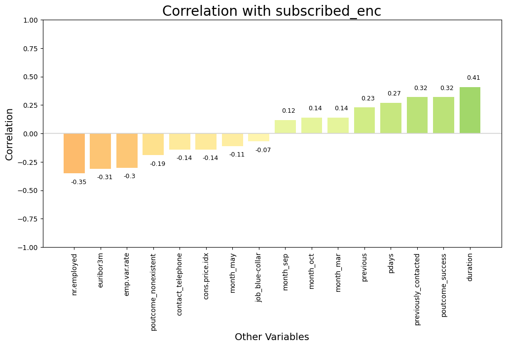
Top Correlations with Target#
Now let’s list and extract the top positive and negative correlations with our target variable.
[21]:
# Get the top positive and negative correlations with the target variable, and save to lists
pos_features, neg_features = dw.get_corr(df_enc, n=15, var='subscribed_enc', return_arrays=True)
Top 15 positive correlations:
Variable 1 Variable 2 Correlation
0 duration subscribed_enc 0.41
1 poutcome_success subscribed_enc 0.32
2 previously_contacted subscribed_enc 0.32
3 pdays subscribed_enc 0.27
4 previous subscribed_enc 0.23
5 month_mar subscribed_enc 0.14
6 month_oct subscribed_enc 0.14
7 month_sep subscribed_enc 0.12
8 no_default_1 subscribed_enc 0.10
9 job_student subscribed_enc 0.09
10 job_retired subscribed_enc 0.09
11 month_dec subscribed_enc 0.08
12 month_apr subscribed_enc 0.08
13 cons.conf.idx subscribed_enc 0.06
14 marital_single subscribed_enc 0.05
Top 15 negative correlations:
Variable 1 Variable 2 Correlation
0 nr.employed subscribed_enc -0.35
1 euribor3m subscribed_enc -0.31
2 emp.var.rate subscribed_enc -0.30
3 poutcome_nonexistent subscribed_enc -0.19
4 contact_telephone subscribed_enc -0.14
5 cons.price.idx subscribed_enc -0.14
6 month_may subscribed_enc -0.11
7 campaign subscribed_enc -0.07
8 job_blue-collar subscribed_enc -0.07
9 education_basic.9y subscribed_enc -0.05
10 marital_married subscribed_enc -0.04
11 month_jul subscribed_enc -0.03
12 job_services subscribed_enc -0.03
13 job_entrepreneur subscribed_enc -0.02
14 day_of_week_mon subscribed_enc -0.02
Plot Correlations#
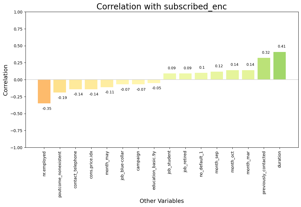
dw.plot_corr() plots the top n correlations of one variable against others in a DataFrame.
This function generates a barplot that visually represents the correlations of a specified column with other numeric columns in a DataFrame. It displays both the strength (height of the bars) and the nature (color) of the correlations (positive or negative). The function computes correlations using the specified method and presents the strongest positive and negative correlations up to the number specified by n. Correlations are ordered from strongest to lowest, from the outside in.
Use this to communicate the correlations of one particular variable (ex: target y) in relation to others with a very clean design. It’s much easier to scan this correlation chart vs. trying to find the variable of interest in a heatmap. The fixed Y axis scales, and Red-Yellow-Green color palette, ensure the actual magnitudes of the positive or negative correlations are clear and not misinterpreted.
[26]:
# Plot a chart showing the top correlations with target variable
dw.plot_corr(df_enc, 'subscribed_enc', n=16, size=(12,6), rotation=90)
Plot 3D Chart#
dw.plot_3d() creates a 3D scatter plot using Plotly Express.
This function generates an interactive 3D scatter plot using the Plotly Express library. It allows for customization of the x, y, and z axes, as well as color coding of the points based on the column specified for color (similar to the hue parameter in Seaborn). A color_discrete_map dictionary can be passed to map specific values of the color column to colors. Alternatively, you can just pass a color_discrete_map or color_continuous_scale depending on the type
of values in the color column. Onlye 1 of these 3 coloring methods should be used at a time. The plot can also be displayed with either a linear or logarithmic scale on each axis by setting x_scale, y_scale, or z_scale from ‘linear’ to ‘log’.
Use this function to visualize and explore relationships between three variables in a dataset, with the option to color code the points based on a fourth variable. It is a great way to visualize the top 3 principal components, dimensioned by the target variable.
[27]:
# Load some PCA data that has good clustering
df_X_scaled_pca_7_XY = pd.read_csv('data/df_X_scaled_pca_7_XY.csv')
[28]:
# Map colors for consistent display of the 'Churn' values
color_map_churn = {'Customer Stayed': px.colors.qualitative.D3[0], 'Customer Left': px.colors.qualitative.D3[1]}
[29]:
# Plot a 3-dimensional chart
dw.plot_3d(df=df_X_scaled_pca_7_XY, x='PCA1', y='PCA2', z='PCA3', color='Churn', color_discrete_map=color_map_churn)
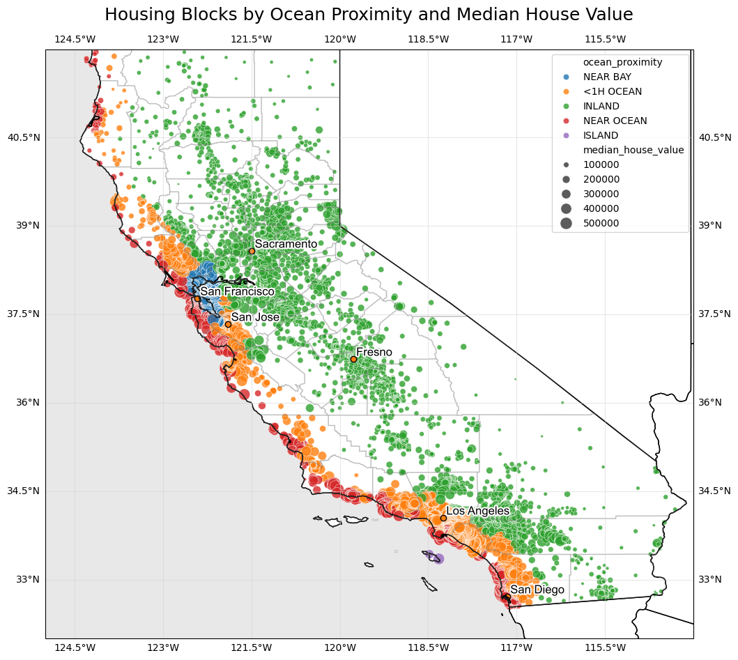
Plot Map of California#
dw.plot_map_ca() plots longitude and latitude data on a geographic map of California.
This function creates a geographic map of California using Cartopy and overlays data points from a DataFrame. The map includes major cities, county boundaries, and geographic terrain features. Specify the columns in the dataframe that map to the longitude (lon) and the latitude (lat). Then specify an optional hue column to see changes in this variable by color, and/or a size column to see changes in this varible by dot size. So two variables can be visualized at once.
A few parameters can be customized, such as the range of the dot sizes (size_range) if you’re using size. You can also just use dot_size to specify a fixed size for all the dots on the map. The alpha transparency can be adjusted, to make sure you at least have a chance of seeing dots of a different color that may be covered up by the top-most layer. You can also customize the color_map for the hue parameter.
Use this function to visualize geospatial data related to California on a clean map.
[30]:
# Load some data with latitude and longitude for California
df_housing = pd.read_csv('data/housing_no_outliers.csv', index_col=0)
[31]:
# Use custom function plot data on California map
dw.plot_map_ca(df_housing, lon='longitude', lat='latitude', hue='ocean_proximity', size='median_house_value', size_range=(5, 150), alpha=0.8, title='Housing Blocks by Ocean Proximity and Median House Value')
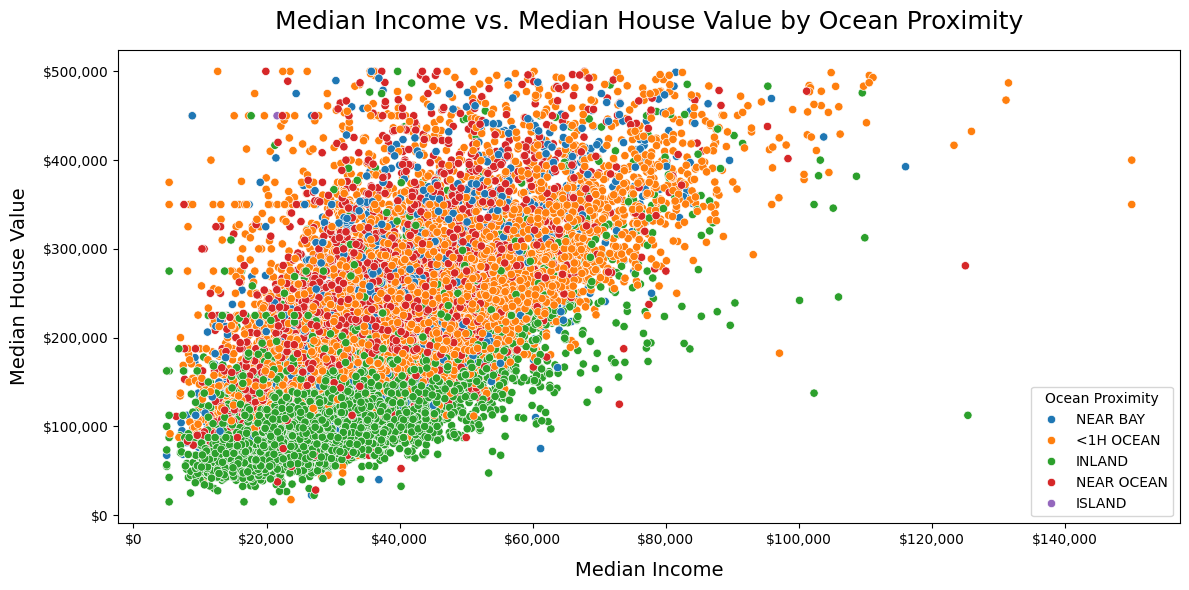
Plot Scatterplot#
dw.plot_scatt() creates a scatter plot using Seaborn’s scatterplot function.
This function generates a scatter plot using the Seaborn library. It allows for customization of the x and y axes, as well as the hue and size dimensions. The hue parameter is used to color the points based on a categorical column, while the size parameter is used to vary the size of the points based on a numerical column or a fixed value. You can also set the range of sizes with size_range, and the title of the plot with title. The alpha parameter controls
the transparency of the points. You can also specify a color map with color_map to change the color scheme of the plot. The fig_size parameter allows you to set the size of the figure.
Use this function to visualize relationships between two variables in a dataset, with the option to color and size the points based on additional variables. It is a great way to explore correlations between variables and identify patterns in the data.
[32]:
# Create a scatterplot of the housing data
dw.plot_scatt(df=df_housing, x='median_income', y='median_house_value', hue='ocean_proximity', x_format='large_dollars', y_format='large_dollars',
title='Median Income vs. Median House Value by Ocean Proximity', x_label='Median Income', y_label='Median House Value',
legend_title='Ocean Proximity')
Print ASCII Image#
dw.print_ascii_image() prints an ASCII representation of one or two PyTorch images.
This function takes one or two PyTorch tensors representing images and prints their ASCII representation. It supports various options to customize the output, such as the number of channels, orientation, and value representation (binary or continuous). The function can also merge multiple channels into a single grayscale representation using either the mean or a weighted sum of the channels.
The tensor data should be concatenated into one long vector. For example, for a single-channel image of size 28x28, the tensor should have a size of [784]. For a three-channel image of size 32x32, the tensor should have a size of [3072]. Please process the tensors before passing them to this function.
Use this function when you want to visualize PyTorch images in the console using ASCII characters, perhaps for debugging during your modeling workflow. For example, you can compare two images side by side (a source image from the x dataset, and the corresponding generated image x_hat).
Load Tensor Images#
[33]:
# Load sample tensor images
image1 = torch.load('data/mnist_28x28_ch1_x0.pt')
image2 = torch.load('data/svhn_32x32_ch3_x0.pt')
image3 = torch.load('data/svhn_32x32_ch3_xhat0.pt')
Review Tensor Data#
This function was designed to work with a single dimension tensor, with no separate channel dimensions. So if you had multiple channels as a 2nd dimension, they would have been already concatenated together. If you have a batch of let’s say [100, 784] to represent 100 images with length 784 (for a 28x28 MNIST image), and that’s your x dataset, you would pass x[0] or x[i] into this function.
[34]:
# Review the dimensions, note there is no batch nor channel dimension, everything is concatenated
print(f"image1 size: {list(image1.size())}")
print(f"image2 size: {list(image2.size())}")
print(f"image3 size: {list(image3.size())}")
image1 size: [784]
image2 size: [3072]
image3 size: [3072]
[35]:
# Sample 28x28 1-channel tensor of '4' from MNIST data
image1
[35]:
tensor([0., 0., 0., 0., 0., 0., 0., 0., 0., 0., 0., 0., 0., 0., 0., 0., 0., 0.,
0., 0., 0., 0., 0., 0., 0., 0., 0., 0., 0., 0., 0., 0., 0., 0., 0., 0.,
0., 0., 0., 0., 0., 0., 0., 0., 0., 0., 0., 0., 0., 0., 0., 0., 0., 0.,
0., 0., 0., 0., 0., 0., 0., 0., 0., 0., 0., 0., 0., 0., 0., 0., 0., 0.,
0., 0., 0., 0., 0., 0., 0., 0., 0., 0., 0., 0., 0., 0., 0., 0., 0., 0.,
0., 0., 0., 0., 0., 0., 0., 0., 0., 0., 0., 0., 0., 0., 0., 0., 0., 0.,
0., 0., 0., 0., 0., 0., 0., 0., 0., 0., 0., 0., 0., 0., 0., 0., 0., 0.,
0., 0., 0., 0., 0., 0., 1., 0., 0., 0., 0., 0., 0., 0., 0., 0., 0., 0.,
0., 0., 0., 0., 0., 0., 0., 1., 1., 0., 0., 0., 0., 0., 0., 1., 1., 0.,
0., 0., 0., 0., 0., 0., 0., 0., 0., 0., 0., 0., 0., 0., 0., 0., 0., 1.,
1., 0., 0., 0., 0., 0., 0., 1., 1., 1., 0., 0., 0., 0., 0., 0., 0., 0.,
0., 0., 0., 0., 0., 0., 0., 0., 0., 1., 1., 0., 0., 0., 0., 0., 0., 0.,
1., 0., 0., 0., 0., 0., 0., 0., 0., 0., 0., 0., 0., 0., 0., 0., 0., 0.,
1., 1., 1., 0., 0., 0., 0., 0., 0., 1., 0., 0., 0., 0., 0., 0., 0., 0.,
0., 0., 0., 0., 0., 0., 0., 0., 0., 1., 1., 1., 0., 0., 0., 0., 0., 0.,
1., 1., 0., 0., 0., 0., 0., 0., 0., 0., 0., 0., 0., 0., 0., 0., 0., 0.,
0., 0., 1., 0., 0., 0., 0., 0., 0., 0., 1., 1., 0., 0., 0., 0., 0., 0.,
0., 0., 0., 0., 0., 0., 0., 0., 0., 0., 0., 0., 1., 0., 0., 0., 0., 0.,
0., 0., 1., 0., 0., 0., 0., 0., 0., 0., 0., 0., 0., 0., 0., 0., 0., 0.,
0., 0., 0., 0., 1., 1., 0., 0., 0., 0., 0., 1., 1., 1., 0., 0., 0., 0.,
0., 0., 0., 0., 0., 0., 0., 0., 0., 0., 0., 0., 0., 0., 1., 1., 0., 0.,
0., 0., 0., 1., 1., 0., 0., 0., 0., 0., 0., 0., 0., 0., 0., 0., 0., 0.,
0., 0., 0., 0., 1., 1., 1., 1., 1., 0., 0., 0., 0., 1., 1., 0., 0., 0.,
0., 0., 0., 0., 0., 0., 0., 0., 0., 0., 0., 0., 0., 0., 1., 1., 1., 1.,
1., 1., 1., 0., 1., 1., 0., 0., 0., 0., 0., 0., 0., 0., 0., 0., 0., 0.,
0., 0., 0., 0., 0., 0., 0., 1., 1., 1., 1., 1., 1., 1., 1., 1., 0., 0.,
1., 1., 0., 0., 0., 0., 0., 0., 0., 0., 0., 0., 0., 0., 0., 0., 0., 1.,
1., 1., 1., 1., 1., 1., 1., 1., 1., 1., 1., 1., 0., 0., 0., 0., 0., 0.,
0., 0., 0., 0., 0., 0., 0., 0., 0., 0., 0., 1., 1., 0., 1., 1., 0., 0.,
0., 0., 1., 0., 0., 0., 0., 0., 0., 0., 0., 0., 0., 0., 0., 0., 0., 0.,
0., 0., 0., 0., 0., 0., 1., 1., 0., 0., 0., 0., 0., 0., 0., 0., 0., 0.,
0., 0., 0., 0., 0., 0., 0., 0., 0., 0., 0., 0., 0., 0., 0., 0., 1., 1.,
0., 0., 0., 0., 0., 0., 0., 0., 0., 0., 0., 0., 0., 0., 0., 0., 0., 0.,
0., 0., 0., 0., 0., 0., 0., 1., 1., 0., 0., 0., 0., 0., 0., 0., 0., 0.,
0., 0., 0., 0., 0., 0., 0., 0., 0., 0., 0., 0., 0., 0., 0., 0., 0., 1.,
1., 1., 0., 0., 0., 0., 0., 0., 0., 0., 0., 0., 0., 0., 0., 0., 0., 0.,
0., 0., 0., 0., 0., 0., 0., 0., 1., 1., 1., 0., 0., 0., 0., 0., 0., 0.,
0., 0., 0., 0., 0., 0., 0., 0., 0., 0., 0., 0., 0., 0., 0., 0., 0., 0.,
0., 0., 0., 0., 0., 0., 0., 0., 0., 0., 0., 0., 0., 0., 0., 0., 0., 0.,
0., 0., 0., 0., 0., 0., 0., 0., 0., 0., 0., 0., 0., 0., 0., 0., 0., 0.,
0., 0., 0., 0., 0., 0., 0., 0., 0., 0., 0., 0., 0., 0., 0., 0., 0., 0.,
0., 0., 0., 0., 0., 0., 0., 0., 0., 0., 0., 0., 0., 0., 0., 0., 0., 0.,
0., 0., 0., 0., 0., 0., 0., 0., 0., 0., 0., 0., 0., 0., 0., 0., 0., 0.,
0., 0., 0., 0., 0., 0., 0., 0., 0., 0.])
[36]:
# Sample 32x32 3-channel tensor of '8' from SVHN data
image2
[36]:
tensor([0.4549, 0.4510, 0.4667, ..., 0.2784, 0.2902, 0.3020])
[37]:
# Sample 32x32 3-channel tensor of '8' from SVHN data (generated)
image3
[37]:
tensor([0.3091, 0.2603, 0.3264, ..., 0.3444, 0.3897, 0.3819])
Print Binary Image#
This converts 0 and 1 to an empty space and a solid block (’█’) to make it easier to scan. A space is added to roughly approximate a square aspect ratio of 28x28 in this example.
[38]:
# Print a single binary image with a space between characters
dw.print_ascii_image(image1, width=28, height=28, add_space=True)
█
█ █ █ █
█ █ █ █ █
█ █ █
█ █ █ █
█ █ █ █ █
█ █ █
█ █
█ █ █ █ █
█ █ █ █
█ █ █ █ █ █ █
█ █ █ █ █ █ █ █ █
█ █ █ █ █ █ █ █ █ █ █
█ █ █ █ █ █ █ █ █ █ █ █ █
█ █ █ █ █
█ █
█ █
█ █
█ █ █
█ █ █
Print Continuous Image with 3 Channels#
For continuous data (floats between 0.00 and 1.00) we need to convert those intensities (or probabilities) into a visual representation. By default, the ascii_chars are ‘@%#*+=-:. ‘, but they can be changed. The characters should be ordered from dark to light, with the last character representing the lightest value.
[39]:
# Print a single continuous image with 3 channels
dw.print_ascii_image(image2, values='continuous', channels=3, width=32, height=32, orientation='horizontal')
++++*#%@@%#*++======+*#%%@@@@%%% ===++*#%@%#+========+*#%%@@%%%%% ----=+*###*+=-------==**#%######
---=+*%@@#*=----::-==+*%%@@@@@%% :-:-=*#%%#+=-:::::--=+*%%@@@@%%% ::::-=*##*+-::....::-=+*#%%#####
::-=+*%@%#+=-----::--=+#%@@@@@%% :::-+*#%%*+-:::-::::-=+#%@@@@%%% ...:-=*##+=::.::....:-=*##%#####
:--=*#%%%*=----==-:::-+*%@@@%%%% ::-=*##%#+=:::-==-:::-+*%@@@%%%# ..:-=+*#*+-:.::--:...:=+*####***
:-=+#%%%%+=::-=++=:::-=*%%@%%%## :--+#%%%#+-:::=++=:::-=*%%@%%%## .::=+**#*=:..:-==-...:-+*###****
:-=*%@@%#=-::-+**=:::-=*%%@%%### :-=*#%%%*=:.:-=**=:.:-=*%@@%%### .:-+*##*+-:..:=++=...:-+*###****
--+#%@@%*=:::-+##+::::=*%@@%#### :-+#%@@%*-:.:-+**+::::=*%@@%#### ::=+###*+:...-=**=:...-=*##*****
:-+#@@@%#=:::=+##+::::=*%%%%#### :-+#%@@%*-:::-+##+::::=*%%%%#### .:=*#%##+:...-+**=:...-=*##**+*+
:-+#@@@%*=:::=*##+:.:-=*%%%%#### :-+#%@%#*-:.:-+##+:::-=*%%%%#### .:=*#%#*+:..:-+##=...:-+*##**+*+
:-+#%@@%#=-:-=+##=:::-+*%%%%%### :-+#%@%#*=:::-+##=:::-+#%%%%%### .:=*###*+-:.:-=**-...:=+*##*****
:-*#%@%%#+=--=+#*=:::-+#%@%%%%%# :-+#%@%#*=-::-+#*=::--+#%@@%%%## :-=*###*+=:::-=*+-..::=+###*****
:-*#%@%%#+=-:-=*+=::-=+#%@%%%%%% :-*#%%%#*+-::-=++=::-=*#%@@%%%%% :-+*###*+=-:.:-==-..::=*###*#***
:=*#@@@@%*=-::-=--:--=*#%%%%%%%% :=*#%@%%#+=-::-=-----=*#%@%%%%%% :-+*#%##*+-:..:-::..:-=**##*#***
:-+#%@@@%*=-::-------=*#%%%%%%%% :-+#%%%%#+=-.:-------=*#%%%%%%%% .:+*#####+-: .::::::::=+****#**#
-=++*%%%#+--:-===+=---=*%%%%%%%% -=++*#%%*=-:::=+++=---+*%%%%%%%# :-==+*##*=::.:-----:.:-+********
--==+*##*-:::=+***=-:-=*#%%%%%%% --==+*#*+-:::=+***=-:-=*#%%%%%## :---=+**=:...-=++=-:..:=********
:--==***+-::-+*##*=-::=*#%%%%%%% :---=+*+=:.:-+*##*=-::=*#%%%%%## ::---+++=:..:=+**+-:..:=+*******
:---=+*+=::-=*#%#*=-:-=*#%%%%%%% ::--=+++-:.:-+#%#*=-:-=*#%%%%%## .:::-=+=-:.:-+***+-:..:=+*******
:::-=++=-::-=*#%#*=-:-=*#%%%%%%% :::--=+=-:::=*###*=-:-=*#%%%%%%# ...:-==-::.:-+***=-:..-=********
:::-=++=-::-=*#%#*=-:-=*#%%%%%%% .::-=++=-:.:=*###+--:-=*#%%%%%%% ...:-==-:..:-+*#*=::.:-=********
:::-=++=-:::=*%%#+-::-=*#%%%%%%% .::-=++-::.:=*###+-::-=*#%%%%%%% ...:-==-:..:-+*#*=:..:-+********
:::-=+=-::::=*##*=-:-=+*#%%%%%%% ..:-=+=-::::=*##*=:::-+*#%%%%%%% ...:-=-:...:-+**+-:..:=+********
::-=++=-:::-=###*=---=+#%%%%%%%% :::=++=-::::=*##+-::-=+#%%%%%%%% ..:-==-:...:-***+-:.:-=+*#*****#
--=+**+-:::-=*##*=:--=*#%@%%%%%% :-=+**+-:.:-=***+-::-=*#%%%%%%%% .:-=++=:...:=+**=-..:-+*###**#*#
-=++*#+-:::-=+**+----=*%%@@%%%%% -==+*#+-:::-=+*+=-::-=*#%@@%%%%# :-==++=:...:-=++-::::-+*######**
==+*##*=::::-=+=----=+*%%@@%%%%% -=+*##*=:.::-===-:--=+*%%@%%%%%# -==+**+-:...:-=-::::-=+*######*#
-=+*##*=-:::-==-:-===*#%@@%%%%%% -=+*##*=:...:-=-::-==+#%%%%%%%%% :-=+**+-:...:--:.::--=*#########
--=+##*+-::::-=---=++*#%@@%%%%%% --=*##*=-::.:-----==+*#%%%%%%%## :-=+**+=:....:-:::--=+*####*####
:--+*##+=--::-====++*##%%%%%%%%# :-=+*#*+=-:::----=++*##%%%%##%## .:-=+*+=-::..:--:-==++*####**##*
::-+*%##+==--==++***##%%%%%%%%%% ::-+*##*+-----=+++**##%%%%%#%%## .:-=+**+=::::--===+++*#####*####
--=*#%%%#+++++*#####%%%@@%%%%@%% --=*#%%#*+++++**#####%%%%%%#%%%% ::-+*##*+=====++*****######*#%##
+++*#%%%##****#######%%%%%%#%%%# +++*#%%%#*****########%%%%###### ===+*###*+++++********####**####
Print Continuous Image with Merged Channels#
This averages the channels together, using perceptual weights by default, which is typical for greyscale conversion. But other channel_weights can be specified.
[40]:
# Print a single continuous image but merge the channels into one:
dw.print_ascii_image(image2, values='continuous', channels=3, width=32, height=32, merge_channels=True, add_space=True)
+ + + + * # % @ @ % # * + + = = = = = = + * # % % @ @ @ @ % % %
- - - = + * % @ @ # * = - - - - : : - = = + * % % @ @ @ @ @ % %
: : - = + * % @ % # + = - - - - - : : - - = + # % @ @ @ @ @ % %
: - - = * # % % % * = - - - - = = - : : : - + * % @ @ @ % % % %
: - = + # % % % % + = : : - = + + = : : : - = * % % @ % % % # #
: - = * % @ @ % # = - : : - + * * = : : : - = * % % @ % % # # #
- - + # % @ @ % * = : : : - + # # + : : : : = * % @ @ % # # # #
: - + # @ @ @ % # = : : : = + # # + : : : : = * % % % % # # # #
: - + # @ @ @ % * = : : : = * # # + : . : - = * % % % % # # # #
: - + # % @ @ % # = - : - = + # # = : : : - + * % % % % % # # #
: - * # % @ % % # + = - - = + # * = : : : - + # % @ % % % % % #
: - * # % @ % % # + = - : - = * + = : : - = + # % @ % % % % % %
: = * # @ @ @ @ % * = - : : - = - - : - - = * # % % % % % % % %
: - + # % @ @ @ % * = - : : - - - - - - - = * # % % % % % % % %
- = + + * % % % # + - - : - = = = + = - - - = * % % % % % % % %
- - = = + * # # * - : : : = + * * * = - : - = * # % % % % % % %
: - - = = * * * + - : : - + * # # * = - : : = * # % % % % % % %
: - - - = + * + = : : - = * # % # * = - : - = * # % % % % % % %
: : : - = + + = - : : - = * # % # * = - : - = * # % % % % % % %
: : : - = + + = - : : - = * # % # * = - : - = * # % % % % % % %
: : : - = + + = - : : : = * % % # + - : : - = * # % % % % % % %
: : : - = + = - : : : : = * # # * = - : - = + * # % % % % % % %
: : - = + + = - : : : - = # # # * = - - - = + # % % % % % % % %
- - = + * * + - : : : - = * # # * = : - - = * # % @ % % % % % %
- = + + * # + - : : : - = + * * + - - - - = * % % @ @ % % % % %
= = + * # # * = : : : : - = + = - - - - = + * % % @ @ % % % % %
- = + * # # * = - : : : - = = - : - = = = * # % @ @ % % % % % %
- - = + # # * + - : : : : - = - - - = + + * # % @ @ % % % % % %
: - - + * # # + = - - : : - = = = = + + * # # % % % % % % % % #
: : - + * % # # + = = - - = = + + * * * # # % % % % % % % % % %
- - = * # % % % # + + + + + * # # # # # % % % @ @ % % % % @ % %
+ + + * # % % % # # * * * * # # # # # # # % % % % % % # % % % #
Print 2 Image Comparison#
This comes in handy when you are evaluating the input image into an Encoder, in comparison with the output image from a Decoder.
[41]:
# Print 2 images side by side with continuous values merged channels
dw.print_ascii_image(image2, image3, values='continuous', channels=3, width=32, height=32,
merge_channels=True, orientation='vertical', add_space=False)
++++*#%@@%#*++======+*#%%@@@@%%% #%##%##%###%######*###%%###%%%#%
---=+*%@@#*=----::-==+*%%@@@@@%% ***##%%%%#####******##%%%%%%%%##
::-=+*%@%#+=-----::--=+#%@@@@@%% ***###%#%%#**+++++++**##%%%%%%%%
:--=*#%%%*=----==-:::-+*%@@@%%%% +****##%#**+=======+++*%%%@@%%%%
:-=+#%%%%+=::-=++=:::-=*%%@%%%## +++*######+=+====-===**#%@%@%%%#
:-=*%@@%#=-::-+**=:::-=*%%@%%### +++*#####*==-===-=--=++%@@@%@%%%
--+#%@@%*=:::-+##+::::=*%@@%#### =++*####*+--=-===+=--=*#@@@%%%#%
:-+#@@@%#=:::=+##+::::=*%%%%#### ==++*#%#++==-==+++=--=*#%@@@%%%%
:-+#@@@%*=:::=*##+:.:-=*%%%%#### ++++**##*+=-==*+*+=--=*#%@@@@%#%
:-+#%@@%#=-:-=+##=:::-+*%%%%%### ++++*#%#*+--=++**+=-=+*#%@@@@%%%
:-*#%@%%#+=--=+#*=:::-+#%@%%%%%# ==+*+###+==-=+****=-==#%%@%@@%%%
:-*#%@%%#+=-:-=*+=::-=+#%@%%%%%% *++**###*====+****====*#@@@@@@%%
:=*#@@@@%*=-::-=--:--=*#%%%%%%%% +=++*##**+===+***+====+#%@@@@%%#
:-+#%@@@%*=-::-------=*#%%%%%%%% ++++*###*+====+=*+=-==+#%@@@@%%#
-=++*%%%#+--:-===+=---=*%%%%%%%% ==+=*###*+=====+++=--=**%@@@@@%%
--==+*##*-:::=+***=-:-=*#%%%%%%% ==++####*++===+++==--=+#%@@@@%%%
:--==***+-::-+*##*=-::=*#%%%%%%% ===+*###*++--=+++==--=+#%@@@@%%%
:---=+*+=::-=*#%#*=-:-=*#%%%%%%% ==++**#**=+=-=++*+=---+*%%@@@@%#
:::-=++=-::-=*#%#*=-:-=*#%%%%%%% =+=+*###*+-=+++*#+==--+*%%@@@%%%
:::-=++=-::-=*#%#*=-:-=*#%%%%%%% +++++*##*+=--=+***+---+#%%@@%%%%
:::-=++=-:::=*%%#+-::-=*#%%%%%%% ++=++*#**+===+*#**+===+#%@@@@%#%
:::-=+=-::::=*##*=-:-=+*#%%%%%%% ++++**##*+=-=++##*+---=*%@@%%%##
::-=++=-:::-=###*=---=+#%%%%%%%% +++++*#**=--=+*##*==--++%@@@%%%#
--=+**+-:::-=*##*=:--=*#%@%%%%%% +++++*#**=---=**#*+---+*#%@@@%##
-=++*#+-:::-=+**+----=*%%@@%%%%% +==++*#**=---=+***==:=+##@@@%%%#
==+*##*=::::-=+=----=+*%%@@%%%%% +=++**#**+---=+*++==-=*#%@@@%#%#
-=+*##*=-:::-==-:-===*#%@@%%%%%% =+++*###*+==--=++==-=+*#%%%@@%#*
--=+##*+-::::-=---=++*#%@@%%%%%% ++++#*###++--==+=====**%%@%@%@%#
:--+*##+=--::-====++*##%%%%%%%%# ++**###%#*++==+==+=++#%%@@%@@@##
::-+*%##+==--==++***##%%%%%%%%%% ***#*#%%##**++++=++**#%%%@@%%%#%
--=*#%%%#+++++*#####%%%@@%%%%@%% *####%%%###**+++**#*##%%%%%%%%%%
+++*#%%%##****#######%%%%%%#%%%# ##*###%%%%%#*##**#####%%%@%%%##%
Clean#
The dw.clean module provides tools to clean data in preparation for modeling. It contains functions to convert data types, convert unites of measurement, convert time values, and reduce multicollinearity.
Convert Data Types - convert_dtypes()
Convert Data Values - convert_data_values()
Convert Time Values - convert_time_values()
Split Outliers - split_outliers()
Reduce Multicollinearity - reduce_multicollinearity()
Convert Data Types#
dw.convert_dtypes() converts specified columns in a DataFrame to the desired data type.
This function converts the data type of the specified columns in the input DataFrame to the desired target data type. It supports both base Python data types (e.g., int, float, str) and Pandas-specific data types (e.g., ‘int64’, ‘float64’, ‘object’, ‘bool’, ‘datetime64’, ‘timedelta[ns]’, ‘category’). If inplace is set to True (default), the conversion is done in place, modifying the original DataFrame. If inplace is False, a new DataFrame with the converted columns is returned. If
show_results is set to True, it will print the results of each successful conversion and any error messages for columns that could not be converted.
Use this function when you need to convert the data types of specific columns in a DataFrame to a consistent target data type, especially when dealing with multiple columns at once and identifying columns that require further data cleaning.
[42]:
# Review data types of our previously identified categorical features
df[cat_columns].info()
<class 'pandas.core.frame.DataFrame'>
RangeIndex: 41188 entries, 0 to 41187
Data columns (total 11 columns):
# Column Non-Null Count Dtype
--- ------ -------------- -----
0 job 41188 non-null object
1 marital 41188 non-null object
2 education 41188 non-null object
3 default 41188 non-null object
4 housing 41188 non-null object
5 loan 41188 non-null object
6 contact 41188 non-null object
7 month 41188 non-null object
8 day_of_week 41188 non-null object
9 poutcome 41188 non-null object
10 y 41188 non-null object
dtypes: object(11)
memory usage: 3.5+ MB
[43]:
# Review data types of our previously identified numeric features
df[num_columns].info()
<class 'pandas.core.frame.DataFrame'>
RangeIndex: 41188 entries, 0 to 41187
Data columns (total 10 columns):
# Column Non-Null Count Dtype
--- ------ -------------- -----
0 age 41188 non-null int64
1 duration 41188 non-null int64
2 campaign 41188 non-null int64
3 pdays 41188 non-null int64
4 previous 41188 non-null int64
5 emp.var.rate 41188 non-null float64
6 cons.price.idx 41188 non-null float64
7 cons.conf.idx 41188 non-null float64
8 euribor3m 41188 non-null float64
9 nr.employed 41188 non-null float64
dtypes: float64(5), int64(5)
memory usage: 3.1 MB
[44]:
# Change all the categorical features to 'category' data type
dw.convert_dtypes(df, cat_columns, 'category')
[45]:
# Review the updated data types for our categorical features
df[cat_columns].info()
<class 'pandas.core.frame.DataFrame'>
RangeIndex: 41188 entries, 0 to 41187
Data columns (total 11 columns):
# Column Non-Null Count Dtype
--- ------ -------------- -----
0 job 41188 non-null category
1 marital 41188 non-null category
2 education 41188 non-null category
3 default 41188 non-null category
4 housing 41188 non-null category
5 loan 41188 non-null category
6 contact 41188 non-null category
7 month 41188 non-null category
8 day_of_week 41188 non-null category
9 poutcome 41188 non-null category
10 y 41188 non-null category
dtypes: category(11)
memory usage: 444.9 KB
[46]:
# Change all the numeric features to 'float' data type
dw.convert_dtypes(df, num_columns, 'float')
[47]:
# Review the updated data types for our numeric features
df[num_columns].info()
<class 'pandas.core.frame.DataFrame'>
RangeIndex: 41188 entries, 0 to 41187
Data columns (total 10 columns):
# Column Non-Null Count Dtype
--- ------ -------------- -----
0 age 41188 non-null float64
1 duration 41188 non-null float64
2 campaign 41188 non-null float64
3 pdays 41188 non-null float64
4 previous 41188 non-null float64
5 emp.var.rate 41188 non-null float64
6 cons.price.idx 41188 non-null float64
7 cons.conf.idx 41188 non-null float64
8 euribor3m 41188 non-null float64
9 nr.employed 41188 non-null float64
dtypes: float64(10)
memory usage: 3.1 MB
Load Data Units and Time Data#
[48]:
# Load data with mixed data units of measurement, and different date/time formats
df_data_time = pd.read_csv('data/df_data_time.csv', index_col=0)
[49]:
# Review the messy data that mixes numbers and strings, mixes units of measurement, the incconsistent syntax, NaNs, and 0's
df_data_time[:10]
[49]:
| A | B | C | D | |
|---|---|---|---|---|
| 0 | 67.12 mB | 5.19 GB | 45161.23615 | 2019-09-11 |
| 1 | 117.02mB | 2.34 GB | 0.00000 | 2019-07-13 |
| 2 | 39.61 MB | 52.94 MB | 45161.23608 | 2021-02-02 |
| 3 | 56.11 giga | 7.97 GB | 45161.21538 | NaN |
| 4 | 9.84 Gigabytes | 26.23 GB | 45160.48826 | 2019-12-23 |
| 5 | NaN | 2.35 GB | 45160.78181 | NaN |
| 6 | 14.37 Gb | 1.31 TB | 45161.23658 | 2020-09-25 |
| 7 | 63.37mb | 2.65 MB | 45139.22113 | 0 |
| 8 | 27.64gb | 25.84 GB | NaN | 2019-05-18 |
| 9 | 0 B | 39.38 GB | 45160.64827 | NaN |
[50]:
# Review the data types, note the objects and lack of datetime formats
df_data_time.info()
<class 'pandas.core.frame.DataFrame'>
Index: 19 entries, 0 to 18
Data columns (total 4 columns):
# Column Non-Null Count Dtype
--- ------ -------------- -----
0 A 18 non-null object
1 B 19 non-null object
2 C 18 non-null float64
3 D 16 non-null object
dtypes: float64(1), object(3)
memory usage: 760.0+ bytes
[51]:
# Crate lists of columns we want to convert
data_columns = ['A', 'B']
time_columns = ['C', 'D']
Convert Data Values#
dw.convert_data_values() converts mixed data values (ex: GB, MB, KB) to a common unit of measurement.
This function converts values in the specified columns of the input DataFrame to the desired target unit. If inplace is set to True, the conversion is done in place, modifying the original DataFrame. If inplace is False (default), a new DataFrame with the converted values is returned. The string suffix is dropped and the column is converted to a float. It handles inconsistent suffix strings, with or without spaces after the numbers (ex: ‘10GB’, ‘10 Gb’). A variety of spelling options are
supported (ex: ‘GB’, ‘Gigabytes’), but you can pass a custom dictionary as conversion_dict if desired. To display a summary of the changes made, set show_results to True.
Use this to clean up messy data that has a variety of units of measurement appended as text strings to the numeric values. The result will be columns with a common unit of measurement as floats (with no text suffixes).
[52]:
# Convert values in specified columns to GB and assign to a new df
df_data = dw.convert_data_values(df_data_time, data_columns, target_unit='GB')
[53]:
# Review the converted data in the new dataframe
df_data[['A','B']][:10]
[53]:
| A | B | |
|---|---|---|
| 0 | 0.065547 | 5.190000 |
| 1 | 0.114277 | 2.340000 |
| 2 | 0.038682 | 0.051699 |
| 3 | 56.110000 | 7.970000 |
| 4 | 9.840000 | 26.230000 |
| 5 | NaN | 2.350000 |
| 6 | 14.370000 | 1341.440000 |
| 7 | 0.061885 | 0.002588 |
| 8 | 27.640000 | 25.840000 |
| 9 | 0.000000 | 39.380000 |
[54]:
# Review the converted data, note the dtype is now float
df_data[['A','B']].info()
<class 'pandas.core.frame.DataFrame'>
Index: 19 entries, 0 to 18
Data columns (total 2 columns):
# Column Non-Null Count Dtype
--- ------ -------------- -----
0 A 18 non-null float64
1 B 19 non-null float64
dtypes: float64(2)
memory usage: 456.0 bytes
[55]:
# Convert data values to MB in place, modifying the existing df, and show a summary of the changes
dw.convert_data_values(df_data_time, data_columns, target_unit='MB', inplace=True, show_results=True, decimal=8)
Original: 67.12 mB -> Converted: 67.12000000 MB
Original: 117.02mB -> Converted: 117.02000000 MB
Original: 39.61 MB -> Converted: 39.61000000 MB
Original: 56.11 giga -> Converted: 57456.64000000 MB
Original: 9.84 Gigabytes -> Converted: 10076.16000000 MB
Original: NaN -> Converted: NaN
Original: 14.37 Gb -> Converted: 14714.88000000 MB
Original: 63.37mb -> Converted: 63.37000000 MB
Original: 27.64gb -> Converted: 28303.36000000 MB
Original: 0 B -> Converted: 0.00000000 MB
Original: 1.2 GB -> Converted: 1228.80000000 MB
Original: 696.27 Mega -> Converted: 696.27000000 MB
Original: 766.18 Megabytes -> Converted: 766.18000000 MB
Original: 868.81 mega -> Converted: 868.81000000 MB
Original: 0B -> Converted: 0.00000000 MB
Original: 150.35 megabyte -> Converted: 150.35000000 MB
Original: 8.88gigabyte -> Converted: 9093.12000000 MB
Original: 0b -> Converted: 0.00000000 MB
Original: 198.58giga -> Converted: 203345.92000000 MB
Original: 5.19 GB -> Converted: 5314.56000000 MB
Original: 2.34 GB -> Converted: 2396.16000000 MB
Original: 52.94 MB -> Converted: 52.94000000 MB
Original: 7.97 GB -> Converted: 8161.28000000 MB
Original: 26.23 GB -> Converted: 26859.52000000 MB
Original: 2.35 GB -> Converted: 2406.40000000 MB
Original: 1.31 TB -> Converted: 1373634.56000000 MB
Original: 2.65 MB -> Converted: 2.65000000 MB
Original: 25.84 GB -> Converted: 26460.16000000 MB
Original: 39.38 GB -> Converted: 40325.12000000 MB
Original: 0 B -> Converted: 0.00000000 MB
Original: 755.21 MB -> Converted: 755.21000000 MB
Original: 10.67 GB -> Converted: 10926.08000000 MB
Original: 354.73 MB -> Converted: 354.73000000 MB
Original: 0 B -> Converted: 0.00000000 MB
Original: 3.27 GB -> Converted: 3348.48000000 MB
Original: 1.57 GB -> Converted: 1607.68000000 MB
Original: 0 B -> Converted: 0.00000000 MB
Original: 312.59 KB -> Converted: 0.30526367 MB
Convert Time Values#
dw.convert_time_values() converts time values in specified columns of a DataFrame to a target format.
This function converts time values in the specified columns of the input DataFrame to the desired target format. If inplace is set to True, the conversion is done in place, modifying the original DataFrame. If inplace is False (default), a new DataFrame with the converted values is returned.
The function can handle time values in various formats, including: 1. Excel serial format (e.g., ‘45161.23458’) 2. String format (e.g., ‘YYYY-MM-DD’) 3. UNIX epoch in milliseconds (e.g., ‘1640304000000.0’)
If your format is not supported, you can define pattern_list as a list of custom datetime patterns.
If zero_to_nan is set to True, values of ‘0’, ‘0.0’, ‘0.00’, 0, 0.0, or 0.00 will be replaced with NaN. Otherwise, zero values will be detected as a Unix Epoch format with value 1970-01-01 00:00:00.
You can use the default target_format of ‘%Y-%m-%d %H:%M:%S’, or specify a different format. To display a summary of the changes made, set show_results to True.
[56]:
# Convert time values in specified columns to the default format
df_time = dw.convert_time_values(df_data_time, time_columns, show_results=True,
zero_to_nan=True)
Original: 45161.23615 (Excel Serial) -> Converted: 2023-08-25 05:40:03
Original: 0.0 (Zero) -> Converted: NaT
Original: 45161.23608 (Excel Serial) -> Converted: 2023-08-25 05:39:57
Original: 45161.21538 (Excel Serial) -> Converted: 2023-08-25 05:10:08
Original: 45160.48826 (Excel Serial) -> Converted: 2023-08-24 11:43:05
Original: 45160.78181 (Excel Serial) -> Converted: 2023-08-24 18:45:48
Original: 45161.23658 (Excel Serial) -> Converted: 2023-08-25 05:40:40
Original: 45139.22113 (Excel Serial) -> Converted: 2023-08-03 05:18:25
Original: nan -> Converted: NaT
Original: 45160.64827 (Excel Serial) -> Converted: 2023-08-24 15:33:30
Original: 45161.2346 (Excel Serial) -> Converted: 2023-08-25 05:37:49
Original: 45160.88611 (Excel Serial) -> Converted: 2023-08-24 21:15:59
Original: 45161.23702 (Excel Serial) -> Converted: 2023-08-25 05:41:18
Original: 45161.23482 (Excel Serial) -> Converted: 2023-08-25 05:38:08
Original: 45155.64277 (Excel Serial) -> Converted: 2023-08-19 15:25:35
Original: 45161.23592 (Excel Serial) -> Converted: 2023-08-25 05:39:43
Original: 45155.85252 (Excel Serial) -> Converted: 2023-08-19 20:27:37
Original: 45160.83184 (Excel Serial) -> Converted: 2023-08-24 19:57:50
Original: 45161.13627 (Excel Serial) -> Converted: 2023-08-25 03:16:13
Original: 2019-09-11 (Standard Datetime String) -> Converted: 2019-09-11 00:00:00
Original: 2019-07-13 (Standard Datetime String) -> Converted: 2019-07-13 00:00:00
Original: 2021-02-02 (Standard Datetime String) -> Converted: 2021-02-02 00:00:00
Original: nan -> Converted: NaT
Original: 2019-12-23 (Standard Datetime String) -> Converted: 2019-12-23 00:00:00
Original: nan -> Converted: NaT
Original: 2020-09-25 (Standard Datetime String) -> Converted: 2020-09-25 00:00:00
Original: 0 (Zero) -> Converted: NaT
Original: 2019-05-18 (Standard Datetime String) -> Converted: 2019-05-18 00:00:00
Original: nan -> Converted: NaT
Original: 2020-12-15 (Standard Datetime String) -> Converted: 2020-12-15 00:00:00
Original: 2021-05-11 (Standard Datetime String) -> Converted: 2021-05-11 00:00:00
Original: 2020-04-30 (Standard Datetime String) -> Converted: 2020-04-30 00:00:00
Original: 2019-04-17 (Standard Datetime String) -> Converted: 2019-04-17 00:00:00
Original: 2019-12-20 (Standard Datetime String) -> Converted: 2019-12-20 00:00:00
Original: 2020-08-19 (Standard Datetime String) -> Converted: 2020-08-19 00:00:00
Original: 2017-11-27 (Standard Datetime String) -> Converted: 2017-11-27 00:00:00
Original: 2020-11-20 (Standard Datetime String) -> Converted: 2020-11-20 00:00:00
Original: 2019-07-18 (Standard Datetime String) -> Converted: 2019-07-18 00:00:00
[57]:
# Review the converted data in the new dataframe, notice the consistent date/time format
df_time[['C','D']][:10]
[57]:
| C | D | |
|---|---|---|
| 0 | 2023-08-25 05:40:03 | 2019-09-11 |
| 1 | NaT | 2019-07-13 |
| 2 | 2023-08-25 05:39:57 | 2021-02-02 |
| 3 | 2023-08-25 05:10:08 | NaT |
| 4 | 2023-08-24 11:43:05 | 2019-12-23 |
| 5 | 2023-08-24 18:45:48 | NaT |
| 6 | 2023-08-25 05:40:40 | 2020-09-25 |
| 7 | 2023-08-03 05:18:25 | NaT |
| 8 | NaT | 2019-05-18 |
| 9 | 2023-08-24 15:33:30 | NaT |
[58]:
# Review the converted data, note the dtype is now a pandas datetime object
df_time[['C','D']].info()
<class 'pandas.core.frame.DataFrame'>
Index: 19 entries, 0 to 18
Data columns (total 2 columns):
# Column Non-Null Count Dtype
--- ------ -------------- -----
0 C 17 non-null datetime64[ns]
1 D 15 non-null datetime64[ns]
dtypes: datetime64[ns](2)
memory usage: 456.0 bytes
Split Outliers#
dw.split_outliers() splits a DataFrame into two based on the presence of outliers.
This function identifies outliers in the specified columns of the input DataFrame using the Interquartile Range (IQR) method. It then splits the DataFrame into two: one containing rows without outliers and another containing only the rows with outliers.
Use this function when you need to separate outliers from the main data for further analysis or processing.
[59]:
# Specify columns we want to evaluate for outliers, this can be any set of numeric columns
skew_columns = ['duration', 'campaign']
[60]:
# Plot histograms of skewed variables, dimensioned by the target variable
dw.plot_charts(df, plot_type='cont', cont_cols=skew_columns, hue='y', multiple='stack')

[61]:
# Split the dataframe based on the default IQR multiplier of 1.5, looking across the specified columns
df_no_outliers, df_outliers = dw.split_outliers(df, columns=skew_columns)
[62]:
# Compare the size of the 2 dataframes
print(f'df_no_outliers: {len(df_no_outliers):,.0f}')
print(f'df_outliers: {len(df_outliers):,.0f}')
df_no_outliers: 35,963
df_outliers: 5,225
[63]:
# Plot histogram of skewed variables, but now in df with no outliers, dimensioned by the target variable
dw.plot_charts(df_no_outliers, plot_type='cont', cont_cols=skew_columns, hue='y', multiple='stack')
Reduce Multicollinearity#
dw.reduce_multicollinearity() reduces multicollinearity in a DataFrame by removing highly correlated features.
This function iteratively evaluates pairs of features in a DataFrame based on their correlation to each other and to a specified target column. If two features are highly correlated (above corr_threshold), the one with the lower correlation to the target column is removed. The number of NaN and/or zero values can also be considered (prefering removal of features with more) by setting consider_nan or consider_zero to True. The threshold for significant differences (diff_threshold)
can also be adjusted. Sometimes it might appear as if the correlations are the same, but it says one is greater. Adjust decimal to a larger number to see more precision in the correlation.
Use this function to remove redundant features, and reduce a large feature set to a smaller one that contains the features most correlated with the target. This should improve the model’s ability to learn from the dataset, improve performance, and increase interpretability of results.
[64]:
# Remove redundant features, keeping the ones with the strongest correlation to target
df_reduced = dw.reduce_multicollinearity(df_enc, 'subscribed_enc', corr_threshold=0.70,
decimal=4, consider_nan=True, consider_zero=True)
Evaluating pair: 'nr.employed' and 'emp.var.rate' (0.91) - 58 kept features
- Correlation with target: 0.3530, 0.2974
- NaN/0 counts: 0, 0
- Keeping 'nr.employed' (higher correlation, lower or equal count)
Evaluating pair: 'nr.employed' and 'euribor3m' (0.95) - 57 kept features
- Correlation with target: 0.3530, 0.3063
- NaN/0 counts: 0, 0
- Keeping 'nr.employed' (higher correlation, lower or equal count)
Evaluating pair: 'previously_contacted' and 'pdays' (0.84) - 56 kept features
- Correlation with target: 0.3236, 0.2657
- NaN/0 counts: 38714, 38729
- Keeping 'previously_contacted' (higher correlation, lower or equal count)
Evaluating pair: 'previously_contacted' and 'poutcome_success' (0.95) - 55 kept features
- Correlation with target: 0.3236, 0.3155
- NaN/0 counts: 38714, 38850
- Keeping 'previously_contacted' (higher correlation, lower or equal count)
Evaluating pair: 'previous' and 'poutcome_nonexistent' (-0.88) - 54 kept features
- Correlation with target: 0.2287, 0.1916
- NaN/0 counts: 34710, 5485
- Keeping 'poutcome_nonexistent' (higher correlation, significant diff: 0.8420 > 0.1000)
Evaluating pair: 'poutcome_nonexistent' and 'poutcome_failure' (-0.85) - 53 kept features
- Correlation with target: 0.1916, 0.0298
- NaN/0 counts: 5485, 36055
- Keeping 'poutcome_nonexistent' (higher correlation, lower or equal count)
Evaluating pair: 'marital_single' and 'marital_married' (-0.77) - 52 kept features
- Correlation with target: 0.0539, 0.0439
- NaN/0 counts: 28907, 15858
- Keeping 'marital_married' (higher correlation, significant diff: 0.4514 > 0.1000)
[65]:
# Plot a chart showing the top correlations with target variable, but with redundant features removed
dw.plot_corr(df_reduced, 'subscribed_enc', n=16, size=(12,6), rotation=90)
Model#
The dw.model module provides tools to streamline data modeling workflows. It contains functions to set up pipelines, iterate over models, and evaluate results.
Create Pipeline - create_pipeline()
Iterate Model - iterate_model()
Create Results DataFrame - create_results_df()
Run Multiple Iterations - iterate_model()
Plot the Results - plot_results()
Plot ACF Residuals - plot_acf_residuals()
Evaluate Classification Model - eval_model()
Compare Models - compare_models()
Compare Binary Classification Models - compare_models()
Plot the Best Models - plot_results()
Compare Multi-Class Classification Models - compare_models()
Create Binary Classification Neural Network - create_nn_binary
Create Multi-Class Classification Neural Network - create_nn_multi()
Plot Training History - plot_train_history()
Create Pipeline#
dw.create_pipeline() creates a custom pipeline for data preprocessing and modeling.
This function allows you to define a custom pipeline by specifying the desired preprocessing steps (imputation, transformation, scaling, feature selection) and the model to use for predictions. Provide the keys for the steps you want to include in the pipeline. If a step is not specified, it will be skipped. The definition of the keys are defined in a configuration dictionary that is passed to the function. If no external configuration is provided, a default one will be used.
imputer_key(str) is selected fromconfig['imputers']transformer_keys(list or str) are selected fromconfig['transformers']scaler_key(str) is selected fromconfig['scalers']selector_key(str) is selected fromconfig['selectors']model_key(str) is selected fromconfig['models']config['no_scale']lists model keys that should not be scaled.config['no_poly']lists models that should not be polynomial transformed.
By default, the sequence of the Pipeline steps are: Imputer > Column Transformer > Scaler > Selector > Model. However, if impute_first is False, the data will be imputed after the column transformations. Scaling will not be done for any Model that is listed in config['no_scale'] (ex: for decision trees, which don’t require scaling).
A column transformer will be created based on the specified transformer_keys. Any number of column transformations can be defined here. For example, you can define transformer_keys = ['ohe', 'poly2', 'log'] to One-Hot Encode some columns, Polynomial transform some columns, and Log transform others. Just define each of these in your config file to reference the appropriate column lists. By default, these will transform the columns passed in as cat_columns or num_columns. But you
may want to apply different transformations to your categorical features. For example, if you One-Hot Encode some, but Ordinal Encode others, you could define separate column lists for these as ‘ohe_columns’ and ‘ord_columns’, and then define transformer_keys in your config dictionary that reference them:
'ohe': (OneHotEncoder(drop='if_binary', handle_unknown='ignore'), ohe_columns),
'ord': (OrdinalEncoder(), ord_columns),
Here is an example of the configuration dictionary structure:
config = {
'imputers': {
'knn_imputer': KNNImputer().set_output(transform='pandas'),
'simple_imputer': SimpleImputer()
},
'transformers': {
'ohe': (OneHotEncoder(drop='if_binary', handle_unknown='ignore'),
cat_columns),
'ord': (OrdinalEncoder(), cat_columns),
'poly2': (PolynomialFeatures(degree=2, include_bias=False),
num_columns),
'log': (FunctionTransformer(np.log1p, validate=True),
num_columns)
},
'scalers': {
'stand': StandardScaler(),
'minmax': MinMaxScaler()
},
'selectors': {
'rfe_logreg': RFE(LogisticRegression(max_iter=max_iter,
random_state=random_state,
class_weight=class_weight)),
'sfs_linreg': SequentialFeatureSelector(LinearRegression())
},
'models': {
'linreg': LinearRegression(),
'logreg': LogisticRegression(max_iter=max_iter,
random_state=random_state,
class_weight=class_weight),
'tree_class': DecisionTreeClassifier(random_state=random_state),
'tree_reg': DecisionTreeRegressor(random_state=random_state)
},
'no_scale': ['tree_class', 'tree_reg'],
'no_poly': ['tree_class', 'tree_reg']
}
Use this function to quickly create a pipeline during model iteration and evaluation. You can easily experiment with different combinations of preprocessing steps and models to find the best performing pipeline. This function is utilized by iterate_model, compare_models, and compare_reg_models to dynamically build pipelines as part of that larger modeling workflow.
[66]:
# Define column lists
cat_columns = ['ocean_proximity']
num_columns = ['longitude', 'latitude', 'housing_median_age','total_rooms', 'total_bedrooms', 'population',
'households', 'median_income']
[67]:
# Create a pipeline with Standard Scaler and Linear Regression
pipeline = dw.create_pipeline(scaler_key='stand', model_key='linreg', cat_columns=cat_columns, num_columns=num_columns)
[68]:
# Review the pipeline
pipeline
[68]:
Pipeline(steps=[('stand', StandardScaler()), ('linreg', LinearRegression())])In a Jupyter environment, please rerun this cell to show the HTML representation or trust the notebook. On GitHub, the HTML representation is unable to render, please try loading this page with nbviewer.org.
Pipeline(steps=[('stand', StandardScaler()), ('linreg', LinearRegression())])StandardScaler()
LinearRegression()
[69]:
# Create a pipeline with One-Hot Encoding, Standard Scaler, and a Logistic Regression model
pipeline = dw.create_pipeline(transformer_keys=['ohe'],
scaler_key='stand',
model_key='logreg',
cat_columns=cat_columns, num_columns=num_columns)
[70]:
# Review the pipeline
pipeline
[70]:
Pipeline(steps=[('ohe',
ColumnTransformer(force_int_remainder_cols=False,
remainder='passthrough',
transformers=[('ohe',
OneHotEncoder(drop='if_binary',
handle_unknown='ignore'),
['ocean_proximity'])])),
('stand', StandardScaler()),
('logreg',
LogisticRegression(max_iter=10000, random_state=42))])In a Jupyter environment, please rerun this cell to show the HTML representation or trust the notebook. On GitHub, the HTML representation is unable to render, please try loading this page with nbviewer.org.
Pipeline(steps=[('ohe',
ColumnTransformer(force_int_remainder_cols=False,
remainder='passthrough',
transformers=[('ohe',
OneHotEncoder(drop='if_binary',
handle_unknown='ignore'),
['ocean_proximity'])])),
('stand', StandardScaler()),
('logreg',
LogisticRegression(max_iter=10000, random_state=42))])ColumnTransformer(force_int_remainder_cols=False, remainder='passthrough',
transformers=[('ohe',
OneHotEncoder(drop='if_binary',
handle_unknown='ignore'),
['ocean_proximity'])])['ocean_proximity']
OneHotEncoder(drop='if_binary', handle_unknown='ignore')
passthrough
StandardScaler()
LogisticRegression(max_iter=10000, random_state=42)
[71]:
# Create a pipeline with KNN Imputer, One-Hot Encoding, Polynomial Transformation, Log Transformation, Standard Scaler,
# and Gradient Boost Regressor for the model
pipeline = dw.create_pipeline(imputer_key='knn_imputer',
transformer_keys=['ohe', 'poly2', 'log'],
scaler_key='stand',
model_key='boost_reg',
cat_columns=cat_columns, num_columns=num_columns)
[72]:
# Review the pipeline
pipeline
[72]:
Pipeline(steps=[('knn_imputer', KNNImputer()),
('ohe_poly2_log',
ColumnTransformer(force_int_remainder_cols=False,
remainder='passthrough',
transformers=[('ohe',
OneHotEncoder(drop='if_binary',
handle_unknown='ignore'),
['ocean_proximity']),
('poly2',
PolynomialFeatures(include_bias=False),
['longitude', 'latitude',
'housing_median_age',
'total_rooms',
'total_bedrooms',
'population', 'households',
'median_income']),
('log',
FunctionTransformer(func=<ufunc 'log1p'>,
validate=True),
['longitude', 'latitude',
'housing_median_age',
'total_rooms',
'total_bedrooms',
'population', 'households',
'median_income'])])),
('stand', StandardScaler()),
('boost_reg', GradientBoostingRegressor(random_state=42))])In a Jupyter environment, please rerun this cell to show the HTML representation or trust the notebook. On GitHub, the HTML representation is unable to render, please try loading this page with nbviewer.org.
Pipeline(steps=[('knn_imputer', KNNImputer()),
('ohe_poly2_log',
ColumnTransformer(force_int_remainder_cols=False,
remainder='passthrough',
transformers=[('ohe',
OneHotEncoder(drop='if_binary',
handle_unknown='ignore'),
['ocean_proximity']),
('poly2',
PolynomialFeatures(include_bias=False),
['longitude', 'latitude',
'housing_median_age',
'total_rooms',
'total_bedrooms',
'population', 'households',
'median_income']),
('log',
FunctionTransformer(func=<ufunc 'log1p'>,
validate=True),
['longitude', 'latitude',
'housing_median_age',
'total_rooms',
'total_bedrooms',
'population', 'households',
'median_income'])])),
('stand', StandardScaler()),
('boost_reg', GradientBoostingRegressor(random_state=42))])KNNImputer()
ColumnTransformer(force_int_remainder_cols=False, remainder='passthrough',
transformers=[('ohe',
OneHotEncoder(drop='if_binary',
handle_unknown='ignore'),
['ocean_proximity']),
('poly2',
PolynomialFeatures(include_bias=False),
['longitude', 'latitude', 'housing_median_age',
'total_rooms', 'total_bedrooms', 'population',
'households', 'median_income']),
('log',
FunctionTransformer(func=<ufunc 'log1p'>,
validate=True),
['longitude', 'latitude', 'housing_median_age',
'total_rooms', 'total_bedrooms', 'population',
'households', 'median_income'])])['ocean_proximity']
OneHotEncoder(drop='if_binary', handle_unknown='ignore')
['longitude', 'latitude', 'housing_median_age', 'total_rooms', 'total_bedrooms', 'population', 'households', 'median_income']
PolynomialFeatures(include_bias=False)
['longitude', 'latitude', 'housing_median_age', 'total_rooms', 'total_bedrooms', 'population', 'households', 'median_income']
FunctionTransformer(func=<ufunc 'log1p'>, validate=True)
passthrough
StandardScaler()
GradientBoostingRegressor(random_state=42)
Iterate Model#
dw.iterate_model() creates and evaluates a model pipeline with specified parameters.
This function creates a pipeline from specified parameters for imputers, column transformers, scalers, feature selectors, and models. Parameters must be defined in a configuration dictionary containing the sections described below. If config is not defined, the create_pipeline function will revert to the default config embedded in its code. After creating the pipeline, it fits the pipeline to the passed training data, and evaluates performance with both test and training data. There are
options to see plots of residuals and actuals vs. predicted, save results to a results_df with user-defined note, display coefficients, calculate permutation feature importance, variance inflation factor (VIF), and perform cross-validation.
create_pipeline is called to create a pipeline from the specified parameters:
imputer_key(str) is selected fromconfig['imputers']transformer_keys(list or str) are selected fromconfig['transformers']scaler_key(str) is selected fromconfig['scalers']selector_key(str) is selected fromconfig['selectors']model_key(str) is selected fromconfig['models']config['no_scale']lists model keys that should not be scaled.config['no_poly']lists models that should not be polynomial transformed.
Here is an example of the configuration dictionary structure. It is based on what create_pipeline requires to assemble the pipeline. But it adds some additional configuration parameters only required by iterate_model, which are params (grid search parameters) and cv (cross-validation parameters):
config = {
'imputers': {
'knn_imputer': KNNImputer().set_output(transform='pandas'),
'simple_imputer': SimpleImputer()
},
'transformers': {
'ohe': (OneHotEncoder(drop='if_binary', handle_unknown='ignore'),
cat_columns),
'ord': (OrdinalEncoder(), cat_columns),
'poly2': (PolynomialFeatures(degree=2, include_bias=False),
num_columns),
'log': (FunctionTransformer(np.log1p, validate=True),
num_columns)
},
'scalers': {
'stand': StandardScaler(),
'minmax': MinMaxScaler()
},
'selectors': {
'rfe_logreg': RFE(LogisticRegression(max_iter=max_iter,
random_state=random_state,
class_weight=class_weight)),
'sfs_linreg': SequentialFeatureSelector(LinearRegression())
},
'models': {
'linreg': LinearRegression(),
'logreg': LogisticRegression(max_iter=max_iter,
random_state=random_state,
class_weight=class_weight),
'tree_class': DecisionTreeClassifier(random_state=random_state),
'tree_reg': DecisionTreeRegressor(random_state=random_state)
},
'no_scale': ['tree_class', 'tree_reg'],
'no_poly': ['tree_class', 'tree_reg'],
'params': {
'sfs': {
'Selector: sfs__n_features_to_select': np.arange(3, 13, 1),
},
'linreg': {
'Model: linreg__fit_intercept': [True],
},
'ridge': {
'Model: ridge__alpha': np.array([0.001, 0.1, 1, 10, 100, 1000, 10000, 100000]),
}
},
'cv': {
'kfold_5': KFold(n_splits=5, shuffle=True, random_state=42),
'kfold_10': KFold(n_splits=10, shuffle=True, random_state=42),
'skf_5': StratifiedKFold(n_splits=5, shuffle=True, random_state=42),
'skf_10': StratifiedKFold(n_splits=10, shuffle=True, random_state=42)
}
}
In addition to the configuration file, you will need to define any column lists if you want to target certain transformations to a subset of columns. For example, you might define a ‘ohe’ transformer for One-Hot Encoding, and reference ‘ohe_columns’ or ‘cat_columns’ in its definition in the config.
When iterate_model completes, it will print out the results and performance metrics, as well as any requested charts. It will return the best model, and also the grid search results (if a grid search was ran). In addition, if save = True it will append the results to a global variable results_df. This should be created using create_results_df beforehand. If export=True it will save the best model to disk using joblib dump with a timestamp.
Use this function to iterate and evaluate different model pipeline configurations, analyze their performance, and select the best model. With one line of code, you can quickly explore a change to the model pipeline, or grid search parameters, and see how it impacts performance. You can also track the results of these iterations in a results_df DataFrame that can be used to evaluate the best model, or to plot the progress you made from each iteration.
Create Results DataFrame#
dw.create_results_df initializes the results_df DataFrame with the columns required for iterate_model.
This function creates a new DataFrame with the following columns: ‘Iteration’, ‘Train MSE’, ‘Test MSE’, ‘Train RMSE’, ‘Test RMSE’, ‘Train MAE’, ‘Test MAE’, ‘Train R^2 Score’, ‘Test R^2 Score’, ‘Pipeline’, ‘Best Grid Params’, ‘Note’, ‘Date’.
Create a results_df with this function, and then pass it as a parameter to iterate_model. The results of each model iteration will be appended to results_df.
[73]:
# Create the dw.results_df required for saving the results of each iteration
results_df = dw.create_results_df()
[74]:
# Show the empty results_df that will store the results of each iteration
results_df
[74]:
| Iteration | Train MSE | Test MSE | Train RMSE | Test RMSE | Train MAE | Test MAE | Train R^2 Score | Test R^2 Score | Pipeline | Best Grid Params | Note | Date |
|---|
Separate X and Y Data#
Let’s prepare the X and y datasets.
[75]:
# Load the California housing dataset
df_housing = pd.read_csv('data/housing_no_outliers.csv', index_col=0)
[76]:
# Define the X and y columns
x_num_columns = ['longitude', 'latitude', 'housing_median_age','total_rooms', 'total_bedrooms', 'population',
'households', 'median_income']
x_cat_columns = ['ocean_proximity']
y_column = ['median_house_value']
[77]:
# Create X and y, with some different combinations of X features
X1 = df_housing[x_num_columns]
X2 = df_housing[x_num_columns + x_cat_columns]
y = df_housing[y_column]
[78]:
# Verify X/Y split
print(f'X1: {X1.shape}, y: {y.shape}')
print(f'X2: {X2.shape}, y: {y.shape}')
X1: (18568, 8), y: (18568, 1)
X2: (18568, 9), y: (18568, 1)
[79]:
# Verify X/Y columns
print(f'X1: ({len(X1.columns)})', list(X1.columns))
print(f'X2: ({len(X2.columns)})', list(X2.columns))
print(f'y: ({len(y.columns)})', list(y.columns))
X1: (8) ['longitude', 'latitude', 'housing_median_age', 'total_rooms', 'total_bedrooms', 'population', 'households', 'median_income']
X2: (9) ['longitude', 'latitude', 'housing_median_age', 'total_rooms', 'total_bedrooms', 'population', 'households', 'median_income', 'ocean_proximity']
y: (1) ['median_house_value']
Split Train and Test Data#
Now we’ll separate the train set from the test set.
[80]:
# Create training and test datasets
X1_train, X1_test, y1_train, y1_test = train_test_split(X1, y, test_size=0.25, random_state=42)
X2_train, X2_test, y2_train, y2_test = train_test_split(X2, y, test_size=0.25, random_state=42)
[81]:
# Verify train/test split
print('X1:', X1_train.shape, X1_test.shape, y1_train.shape, y1_test.shape)
print('X2:', X2_train.shape, X2_test.shape, y2_train.shape, y2_test.shape)
X1: (13926, 8) (4642, 8) (13926, 1) (4642, 1)
X2: (13926, 9) (4642, 9) (13926, 1) (4642, 1)
Create Custom Configuration#
You need to define a configuration dictionary that is structured with names that iterate_model and create_pipeline expect. The format is documented in the docstrings for both of those functions. In addition, you have to import any libraries referenced in the configuration. And some column lists and variables referenced in the configurations need to be defined.
[82]:
# Any column lists referenced in the configuration file need to be defined
cat_columns = ['ocean_proximity']
num_columns = ['longitude', 'latitude', 'housing_median_age','total_rooms', 'total_bedrooms', 'population',
'households', 'median_income']
ohe_columns = cat_columns
ord_columns = cat_columns
poly2_columns = ['median_income']
poly3_columns = ['median_income']
log_columns = ['total_rooms','total_bedrooms','population','households']
[83]:
# If you are doing one-hot encoding, you might want to specify a value to drop
ohe_drop_categories = ['ISLAND']
[84]:
# If you are doing ordinal encoding, the ordering needs to be specified
# Island > Near Bay > Near Ocean > 1 Hour to Ocean > Inland
ocean_proximity_order = [['INLAND', '<1H OCEAN', 'NEAR OCEAN', 'NEAR BAY', 'ISLAND']]
[85]:
# If you want to set any variables in the configurations globally, set them here
max_iter = 1000
random_state = 42
class_weight = 'balanced'
[86]:
# Create a custom configuration file
my_config = {
'imputers': {
'knn_imputer': KNNImputer().set_output(transform='pandas'),
'simple_imputer': SimpleImputer()
},
'transformers': {
'ohe': (OneHotEncoder(drop='if_binary', handle_unknown='ignore'),
ohe_columns),
'ohe_drop': (OneHotEncoder(drop=ohe_drop_categories, handle_unknown='ignore'), ohe_columns),
'ord': (OrdinalEncoder(categories=ocean_proximity_order), ord_columns),
'poly2': (PolynomialFeatures(degree=2, include_bias=False),
poly2_columns),
'poly3': (PolynomialFeatures(degree=3, include_bias=False),
poly3_columns),
'log': (LogTransformer(),
log_columns)
},
'scalers': {
'stand': StandardScaler(),
'minmax': MinMaxScaler()
},
'selectors': {
'rfe_logreg': RFE(LogisticRegression(max_iter=max_iter,
random_state=random_state,
class_weight=class_weight)),
'rfe_linreg': RFE(LinearRegression()),
'sfs_linreg': SequentialFeatureSelector(LinearRegression())
},
'models': {
'linreg': LinearRegression(),
'ridge': Ridge(),
'logreg': LogisticRegression(max_iter=max_iter,
random_state=random_state,
class_weight=class_weight),
'tree_class': DecisionTreeClassifier(random_state=random_state),
'tree_reg': DecisionTreeRegressor(random_state=random_state)
},
'no_scale': ['tree_class', 'tree_reg'],
'no_poly': ['tree_class', 'tree_reg'],
'params': {
'sfs_linreg': {
'sfs_linreg__n_features_to_select': np.arange(5, 10, 1),
},
'rfe_linreg': {
'rfe_linreg__n_features_to_select': np.arange(5, 10, 1),
},
'linreg': {
'linreg__fit_intercept': [True],
},
'ridge': {
'ridge__alpha': np.array([0.001, 0.1, 1, 10, 100, 1000, 10000, 100000]),
},
'tree_reg': {
'tree_reg__max_depth': [3, 5, 7],
'tree_reg__min_samples_split': [5, 10, 15],
'tree_reg__criterion': ['poisson', 'friedman_mse', 'squared_error', 'absolute_error'],
'tree_reg__min_samples_leaf': [2, 4, 6]
}
},
'cv': {
'kfold_5': KFold(n_splits=5, shuffle=True, random_state=42),
'kfold_10': KFold(n_splits=10, shuffle=True, random_state=42),
'skf_5': StratifiedKFold(n_splits=5, shuffle=True, random_state=42),
'skf_10': StratifiedKFold(n_splits=10, shuffle=True, random_state=42)
}
}
[87]:
# Review the configuration, notice the names of the columns and categories have been embedded
my_config
[87]:
{'imputers': {'knn_imputer': KNNImputer(), 'simple_imputer': SimpleImputer()},
'transformers': {'ohe': (OneHotEncoder(drop='if_binary', handle_unknown='ignore'),
['ocean_proximity']),
'ohe_drop': (OneHotEncoder(drop=['ISLAND'], handle_unknown='ignore'),
['ocean_proximity']),
'ord': (OrdinalEncoder(categories=[['INLAND', '<1H OCEAN', 'NEAR OCEAN', 'NEAR BAY',
'ISLAND']]),
['ocean_proximity']),
'poly2': (PolynomialFeatures(include_bias=False), ['median_income']),
'poly3': (PolynomialFeatures(degree=3, include_bias=False),
['median_income']),
'log': (LogTransformer(),
['total_rooms', 'total_bedrooms', 'population', 'households'])},
'scalers': {'stand': StandardScaler(), 'minmax': MinMaxScaler()},
'selectors': {'rfe_logreg': RFE(estimator=LogisticRegression(class_weight='balanced', max_iter=1000,
random_state=42)),
'rfe_linreg': RFE(estimator=LinearRegression()),
'sfs_linreg': SequentialFeatureSelector(estimator=LinearRegression())},
'models': {'linreg': LinearRegression(),
'ridge': Ridge(),
'logreg': LogisticRegression(class_weight='balanced', max_iter=1000, random_state=42),
'tree_class': DecisionTreeClassifier(random_state=42),
'tree_reg': DecisionTreeRegressor(random_state=42)},
'no_scale': ['tree_class', 'tree_reg'],
'no_poly': ['tree_class', 'tree_reg'],
'params': {'sfs_linreg': {'sfs_linreg__n_features_to_select': array([5, 6, 7, 8, 9])},
'rfe_linreg': {'rfe_linreg__n_features_to_select': array([5, 6, 7, 8, 9])},
'linreg': {'linreg__fit_intercept': [True]},
'ridge': {'ridge__alpha': array([1.e-03, 1.e-01, 1.e+00, 1.e+01, 1.e+02, 1.e+03, 1.e+04, 1.e+05])},
'tree_reg': {'tree_reg__max_depth': [3, 5, 7],
'tree_reg__min_samples_split': [5, 10, 15],
'tree_reg__criterion': ['poisson',
'friedman_mse',
'squared_error',
'absolute_error'],
'tree_reg__min_samples_leaf': [2, 4, 6]}},
'cv': {'kfold_5': KFold(n_splits=5, random_state=42, shuffle=True),
'kfold_10': KFold(n_splits=10, random_state=42, shuffle=True),
'skf_5': StratifiedKFold(n_splits=5, random_state=42, shuffle=True),
'skf_10': StratifiedKFold(n_splits=10, random_state=42, shuffle=True)}}
Run Multiple Iterations#
Now that we have our results_df ready to store results, and our configuration is complete, let’s start with a simple model, and then progressively get more complex.
Iteration 1: Linear Regression#
[88]:
# Start with a simple Linear Regression baseline
results_df, iteration_1 = dw.iterate_model(X1_train, X1_test, y1_train, y1_test,
model='linreg',
iteration='1', note='X1. Baseline. Test size: 0.25, Pipeline: LinReg',
plot=True, lowess=True, coef=True, perm=True, vif=True, decimal=2,
save=True, save_df=results_df, config=my_config)
ITERATION 1 RESULTS
Pipeline: linreg
Note: X1. Baseline. Test size: 0.25, Pipeline: LinReg
May 30, 2024 09:17 AM UTC
Predictions:
Train Test
MSE: 3,568,722,086.53 3,614,822,636.93
RMSE: 59,738.78 60,123.40
MAE: 44,353.86 44,484.81
R^2 Score: 0.61 0.62
Permutation Feature Importance:
Feature Importance Mean Importance Std
latitude 1.50 0.01
longitude 1.29 0.01
median_income 0.83 0.01
population 0.29 0.01
total_bedrooms 0.29 0.00
households 0.12 0.00
total_rooms 0.08 0.00
housing_median_age 0.02 0.00
Variance Inflation Factor:
Features VIF Multicollinearity
total_bedrooms 32.40 High
households 30.01 High
total_rooms 13.80 High
latitude 8.74 Moderate
longitude 8.43 Moderate
population 6.75 Moderate
median_income 1.83 Low
housing_median_age 1.30 Low
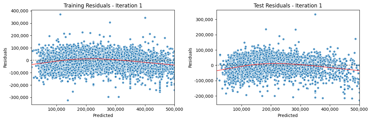
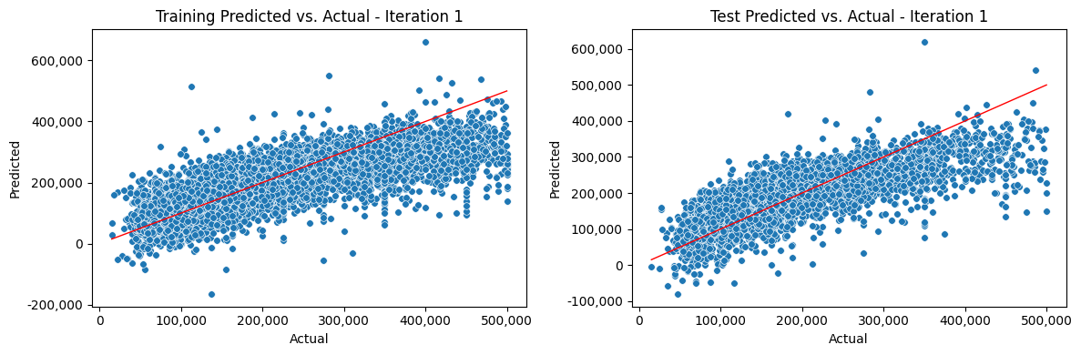
Coefficients:
Feature Coefficient
1 longitude -38,839.33
2 latitude -38,580.35
3 housing_median_age 738.05
4 total_rooms -8.95
5 total_bedrooms 86.41
6 population -33.20
7 households 62.66
8 median_income 3.91
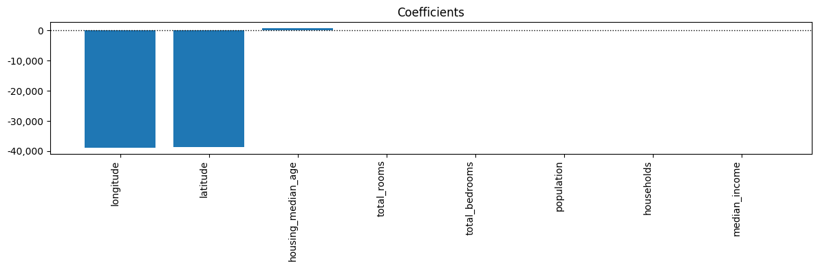
[89]:
# Review the pipeline
iteration_1
[89]:
Pipeline(steps=[('linreg', LinearRegression())])In a Jupyter environment, please rerun this cell to show the HTML representation or trust the notebook. On GitHub, the HTML representation is unable to render, please try loading this page with nbviewer.org.
Pipeline(steps=[('linreg', LinearRegression())])LinearRegression()
Iteration 2: Linear Regression with Log#
[90]:
# Now let's add some log transformation
results_df, iteration_2 = dw.iterate_model(X1_train, X1_test, y1_train, y1_test,
transformers=['log'], model='linreg',
iteration='2', note='X1. Test size: 0.25, Pipeline: Log > LinReg',
plot=True, lowess=True, coef=True, perm=True, vif=True, decimal=2,
save=True, save_df=results_df, config=my_config)
ITERATION 2 RESULTS
Pipeline: log -> linreg
Note: X1. Test size: 0.25, Pipeline: Log > LinReg
May 30, 2024 09:17 AM UTC
Predictions:
Train Test
MSE: 3,333,110,642.12 3,356,136,122.95
RMSE: 57,733.10 57,932.17
MAE: 42,497.76 42,620.51
R^2 Score: 0.63 0.64
Permutation Feature Importance:
Feature Importance Mean Importance Std
latitude 1.37 0.01
longitude 1.17 0.01
total_bedrooms 1.10 0.01
median_income 1.04 0.01
population 0.61 0.01
total_rooms 0.48 0.01
households 0.20 0.00
housing_median_age 0.02 0.00
Variance Inflation Factor:
Features VIF Multicollinearity
total_bedrooms 32.40 High
households 30.01 High
total_rooms 13.80 High
latitude 8.74 Moderate
longitude 8.43 Moderate
population 6.75 Moderate
median_income 1.83 Low
housing_median_age 1.30 Low
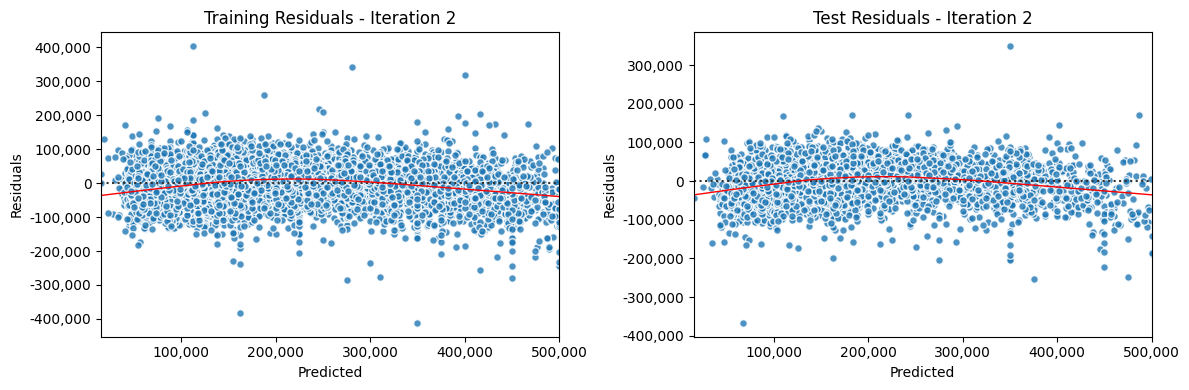
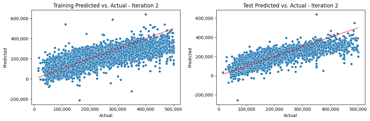
Coefficients:
Feature Coefficient
1 total_rooms_log -63,173.70
2 total_bedrooms_log 99,367.25
3 population_log -72,634.41
4 households_log 42,917.09
5 longitude -36,985.09
6 latitude -36,881.30
7 housing_median_age 810.44
8 median_income 4.37
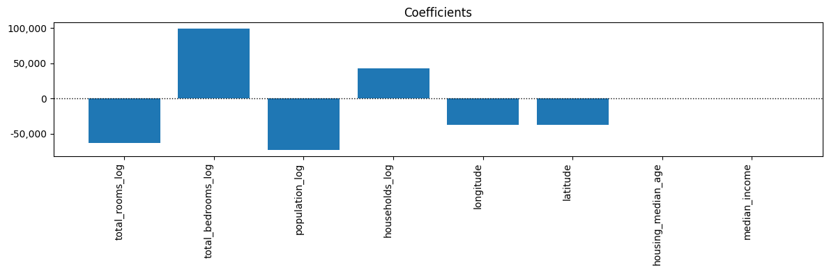
[91]:
# Review the pipeline
iteration_2
[91]:
Pipeline(steps=[('log',
ColumnTransformer(force_int_remainder_cols=False,
remainder='passthrough',
transformers=[('log', LogTransformer(),
['total_rooms',
'total_bedrooms',
'population',
'households'])])),
('linreg', LinearRegression())])In a Jupyter environment, please rerun this cell to show the HTML representation or trust the notebook. On GitHub, the HTML representation is unable to render, please try loading this page with nbviewer.org.
Pipeline(steps=[('log',
ColumnTransformer(force_int_remainder_cols=False,
remainder='passthrough',
transformers=[('log', LogTransformer(),
['total_rooms',
'total_bedrooms',
'population',
'households'])])),
('linreg', LinearRegression())])ColumnTransformer(force_int_remainder_cols=False, remainder='passthrough',
transformers=[('log', LogTransformer(),
['total_rooms', 'total_bedrooms', 'population',
'households'])])['total_rooms', 'total_bedrooms', 'population', 'households']
LogTransformer()
['longitude', 'latitude', 'housing_median_age', 'median_income']
passthrough
LinearRegression()
Iteration 3: Linear Regression with Log, Poly2#
[92]:
# Let's now try adding a polynomial transformation
results_df, iteration_3 = dw.iterate_model(X1_train, X1_test, y1_train, y1_test,
transformers=['log', 'poly2'], model='linreg',
iteration='3', note='X1. Test size: 0.25, Pipeline: Log > Poly2 > LinReg',
plot=True, lowess=True, coef=True, perm=True, vif=True, decimal=2,
save=True, save_df=results_df, config=my_config)
ITERATION 3 RESULTS
Pipeline: log_poly2 -> linreg
Note: X1. Test size: 0.25, Pipeline: Log > Poly2 > LinReg
May 30, 2024 09:17 AM UTC
Predictions:
Train Test
MSE: 3,329,236,889.32 3,350,722,399.55
RMSE: 57,699.54 57,885.42
MAE: 42,383.21 42,493.32
R^2 Score: 0.63 0.64
Permutation Feature Importance:
Feature Importance Mean Importance Std
latitude 1.40 0.01
longitude 1.20 0.01
total_bedrooms 1.04 0.01
median_income 1.02 0.01
population 0.62 0.01
total_rooms 0.43 0.01
households 0.21 0.00
housing_median_age 0.02 0.00
Variance Inflation Factor:
Features VIF Multicollinearity
total_bedrooms 32.40 High
households 30.01 High
total_rooms 13.80 High
latitude 8.74 Moderate
longitude 8.43 Moderate
population 6.75 Moderate
median_income 1.83 Low
housing_median_age 1.30 Low
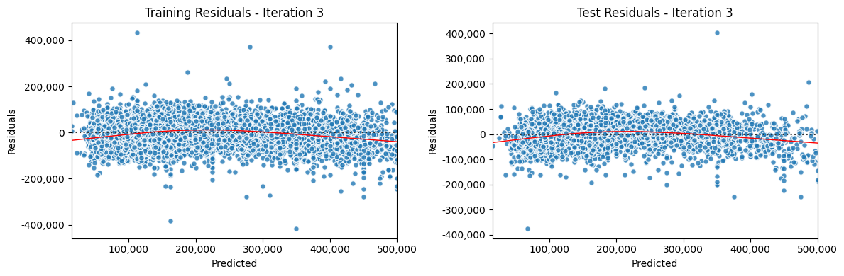

Coefficients:
Feature Coefficient
1 total_rooms_log -60,286.63
2 total_bedrooms_log 96,715.51
3 population_log -73,240.50
4 households_log 43,616.79
5 median_income 3.88
6 median_income^2 0.00
7 longitude -37,366.74
8 latitude -37,286.13
9 housing_median_age 812.71
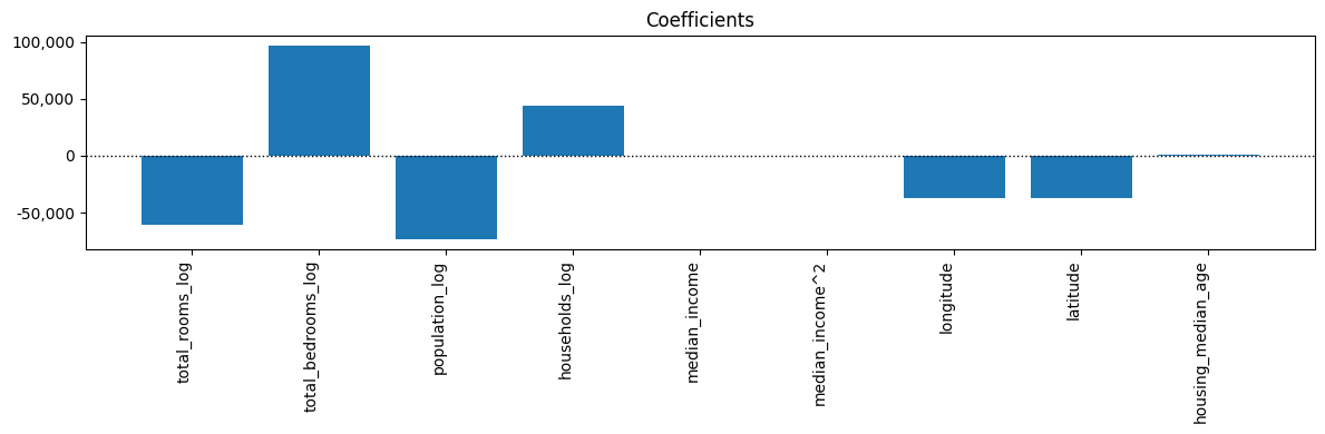
[93]:
# Review the pipeline
iteration_3
[93]:
Pipeline(steps=[('log_poly2',
ColumnTransformer(force_int_remainder_cols=False,
remainder='passthrough',
transformers=[('log', LogTransformer(),
['total_rooms',
'total_bedrooms',
'population',
'households']),
('poly2',
PolynomialFeatures(include_bias=False),
['median_income'])])),
('linreg', LinearRegression())])In a Jupyter environment, please rerun this cell to show the HTML representation or trust the notebook. On GitHub, the HTML representation is unable to render, please try loading this page with nbviewer.org.
Pipeline(steps=[('log_poly2',
ColumnTransformer(force_int_remainder_cols=False,
remainder='passthrough',
transformers=[('log', LogTransformer(),
['total_rooms',
'total_bedrooms',
'population',
'households']),
('poly2',
PolynomialFeatures(include_bias=False),
['median_income'])])),
('linreg', LinearRegression())])ColumnTransformer(force_int_remainder_cols=False, remainder='passthrough',
transformers=[('log', LogTransformer(),
['total_rooms', 'total_bedrooms', 'population',
'households']),
('poly2',
PolynomialFeatures(include_bias=False),
['median_income'])])['total_rooms', 'total_bedrooms', 'population', 'households']
LogTransformer()
['median_income']
PolynomialFeatures(include_bias=False)
['longitude', 'latitude', 'housing_median_age']
passthrough
LinearRegression()
Iteration 4: Linear Regression with OHE, Log, Poly2#
[94]:
# Let's see if one-hot encoding the categorical feature 'ocean_proximity' helps
results_df, iteration_4 = dw.iterate_model(X2_train, X2_test, y2_train, y2_test,
transformers=['ohe', 'log', 'poly2'], model='linreg',
iteration='4', note='X2. Test size: 0.25, Pipeline: OHE > Log > Poly2 > LinReg',
plot=True, lowess=True, coef=True, perm=True, vif=True, decimal=2,
save=True, save_df=results_df, config=my_config)
ITERATION 4 RESULTS
Pipeline: ohe_log_poly2 -> linreg
Note: X2. Test size: 0.25, Pipeline: OHE > Log > Poly2 > LinReg
May 30, 2024 09:17 AM UTC
Predictions:
Train Test
MSE: 3,231,250,156.15 3,242,416,485.65
RMSE: 56,844.09 56,942.22
MAE: 41,276.18 41,406.32
R^2 Score: 0.64 0.66
Permutation Feature Importance:
Feature Importance Mean Importance Std
median_income 0.92 0.01
total_bedrooms 0.72 0.01
population 0.61 0.01
latitude 0.61 0.01
longitude 0.59 0.01
total_rooms 0.26 0.01
households 0.23 0.00
ocean_proximity 0.06 0.00
housing_median_age 0.02 0.00
Variance Inflation Factor:
Features VIF Multicollinearity
total_bedrooms 32.40 High
households 30.01 High
total_rooms 13.80 High
latitude 8.74 Moderate
longitude 8.43 Moderate
population 6.75 Moderate
median_income 1.83 Low
housing_median_age 1.30 Low
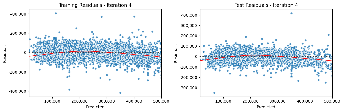
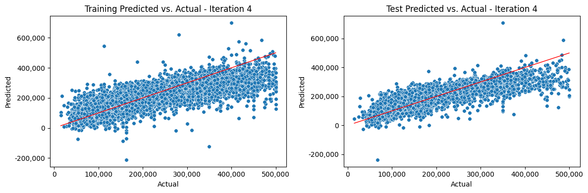
Coefficients:
Feature Coefficient
1 ocean_proximity_<1H OCEAN -4,421.89
2 ocean_proximity_INLAND -38,314.09
3 ocean_proximity_ISLAND 69,133.27
4 ocean_proximity_NEAR BAY -23,189.14
5 ocean_proximity_NEAR OCEAN -3,208.17
6 total_rooms_log -46,665.44
7 total_bedrooms_log 80,641.63
8 population_log -72,784.50
9 households_log 45,310.14
10 median_income 3.54
11 median_income^2 0.00
12 longitude -26,238.41
13 latitude -24,484.78
14 housing_median_age 730.23
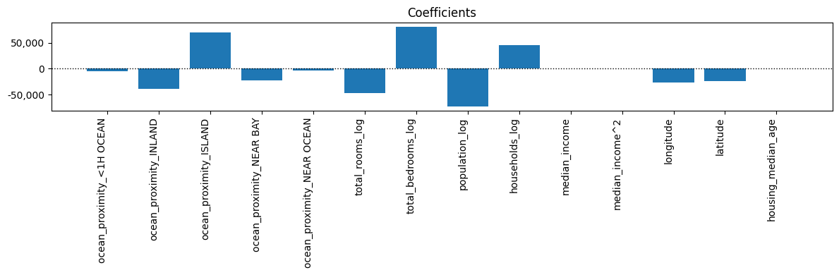
[95]:
# Review the pipeline
iteration_4
[95]:
Pipeline(steps=[('ohe_log_poly2',
ColumnTransformer(force_int_remainder_cols=False,
remainder='passthrough',
transformers=[('ohe',
OneHotEncoder(drop='if_binary',
handle_unknown='ignore'),
['ocean_proximity']),
('log', LogTransformer(),
['total_rooms',
'total_bedrooms',
'population',
'households']),
('poly2',
PolynomialFeatures(include_bias=False),
['median_income'])])),
('linreg', LinearRegression())])In a Jupyter environment, please rerun this cell to show the HTML representation or trust the notebook. On GitHub, the HTML representation is unable to render, please try loading this page with nbviewer.org.
Pipeline(steps=[('ohe_log_poly2',
ColumnTransformer(force_int_remainder_cols=False,
remainder='passthrough',
transformers=[('ohe',
OneHotEncoder(drop='if_binary',
handle_unknown='ignore'),
['ocean_proximity']),
('log', LogTransformer(),
['total_rooms',
'total_bedrooms',
'population',
'households']),
('poly2',
PolynomialFeatures(include_bias=False),
['median_income'])])),
('linreg', LinearRegression())])ColumnTransformer(force_int_remainder_cols=False, remainder='passthrough',
transformers=[('ohe',
OneHotEncoder(drop='if_binary',
handle_unknown='ignore'),
['ocean_proximity']),
('log', LogTransformer(),
['total_rooms', 'total_bedrooms', 'population',
'households']),
('poly2',
PolynomialFeatures(include_bias=False),
['median_income'])])['ocean_proximity']
OneHotEncoder(drop='if_binary', handle_unknown='ignore')
['total_rooms', 'total_bedrooms', 'population', 'households']
LogTransformer()
['median_income']
PolynomialFeatures(include_bias=False)
['longitude', 'latitude', 'housing_median_age']
passthrough
LinearRegression()
Iteration 5: Linear Regression with Ordinal, Log, Poly2#
[96]:
# For one last try, let's see if ordinal encoding 'ocean_proximity' is better
results_df, iteration_5 = dw.iterate_model(X2_train, X2_test, y2_train, y2_test,
transformers=['ord', 'log', 'poly2'], model='linreg',
iteration='5', note='X2. Test size: 0.25, Pipeline: Ord > Log > Poly2 > LinReg',
plot=True, lowess=True, coef=True, perm=True, vif=True, decimal=2,
save=True, save_df=results_df, config=my_config)
ITERATION 5 RESULTS
Pipeline: ord_log_poly2 -> linreg
Note: X2. Test size: 0.25, Pipeline: Ord > Log > Poly2 > LinReg
May 30, 2024 09:17 AM UTC
Predictions:
Train Test
MSE: 3,323,311,153.49 3,339,547,363.35
RMSE: 57,648.17 57,788.82
MAE: 42,307.00 42,378.78
R^2 Score: 0.63 0.65
Permutation Feature Importance:
Feature Importance Mean Importance Std
latitude 1.22 0.01
longitude 1.02 0.01
median_income 1.01 0.01
total_bedrooms 0.99 0.01
population 0.59 0.01
total_rooms 0.41 0.01
households 0.21 0.00
housing_median_age 0.02 0.00
ocean_proximity 0.00 0.00
Variance Inflation Factor:
Features VIF Multicollinearity
total_bedrooms 32.40 High
households 30.01 High
total_rooms 13.80 High
latitude 8.74 Moderate
longitude 8.43 Moderate
population 6.75 Moderate
median_income 1.83 Low
housing_median_age 1.30 Low
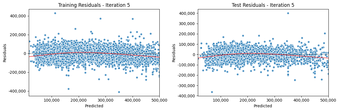
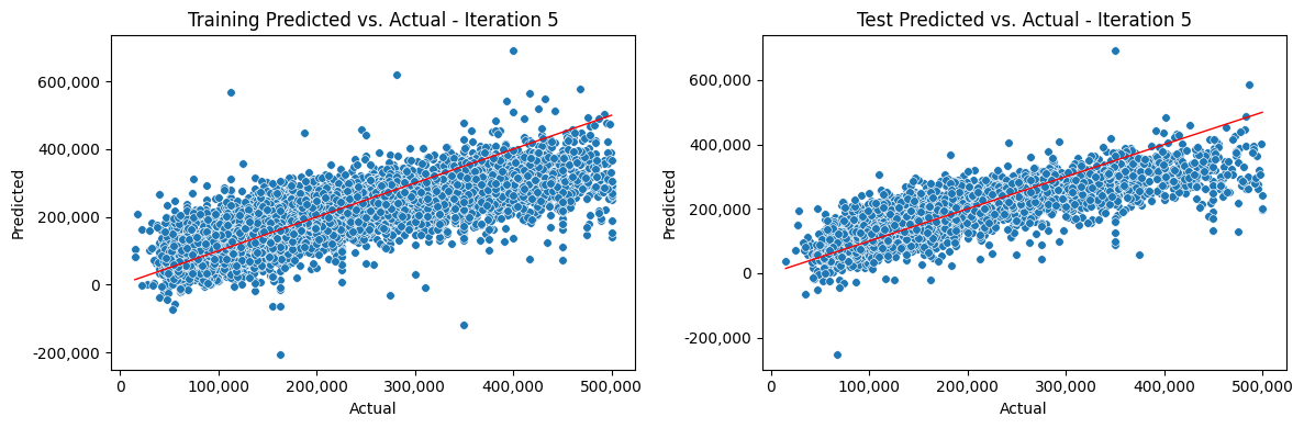
Coefficients:
Feature Coefficient
1 ocean_proximity 3,815.27
2 total_rooms_log -58,936.46
3 total_bedrooms_log 94,196.95
4 population_log -72,001.58
5 households_log 43,435.62
6 median_income 3.86
7 median_income^2 0.00
8 longitude -34,484.02
9 latitude -34,728.43
10 housing_median_age 783.22
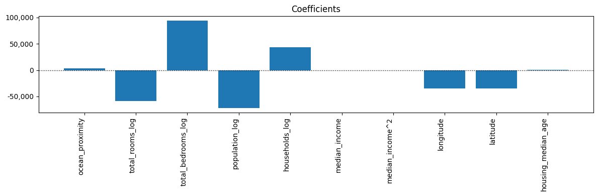
[97]:
# Review the pipeline
iteration_5
[97]:
Pipeline(steps=[('ord_log_poly2',
ColumnTransformer(force_int_remainder_cols=False,
remainder='passthrough',
transformers=[('ord',
OrdinalEncoder(categories=[['INLAND',
'<1H '
'OCEAN',
'NEAR '
'OCEAN',
'NEAR '
'BAY',
'ISLAND']]),
['ocean_proximity']),
('log', LogTransformer(),
['total_rooms',
'total_bedrooms',
'population',
'households']),
('poly2',
PolynomialFeatures(include_bias=False),
['median_income'])])),
('linreg', LinearRegression())])In a Jupyter environment, please rerun this cell to show the HTML representation or trust the notebook. On GitHub, the HTML representation is unable to render, please try loading this page with nbviewer.org.
Pipeline(steps=[('ord_log_poly2',
ColumnTransformer(force_int_remainder_cols=False,
remainder='passthrough',
transformers=[('ord',
OrdinalEncoder(categories=[['INLAND',
'<1H '
'OCEAN',
'NEAR '
'OCEAN',
'NEAR '
'BAY',
'ISLAND']]),
['ocean_proximity']),
('log', LogTransformer(),
['total_rooms',
'total_bedrooms',
'population',
'households']),
('poly2',
PolynomialFeatures(include_bias=False),
['median_income'])])),
('linreg', LinearRegression())])ColumnTransformer(force_int_remainder_cols=False, remainder='passthrough',
transformers=[('ord',
OrdinalEncoder(categories=[['INLAND',
'<1H OCEAN',
'NEAR OCEAN',
'NEAR BAY',
'ISLAND']]),
['ocean_proximity']),
('log', LogTransformer(),
['total_rooms', 'total_bedrooms', 'population',
'households']),
('poly2',
PolynomialFeatures(include_bias=False),
['median_income'])])['ocean_proximity']
OrdinalEncoder(categories=[['INLAND', '<1H OCEAN', 'NEAR OCEAN', 'NEAR BAY',
'ISLAND']])['total_rooms', 'total_bedrooms', 'population', 'households']
LogTransformer()
['median_income']
PolynomialFeatures(include_bias=False)
['longitude', 'latitude', 'housing_median_age']
passthrough
LinearRegression()
Iteration 6: Linear Regression with OHE, Log, Poly3#
[98]:
# One other idea is to see what a 3-degree polynomial does on 'median_income'
results_df, iteration_6 = dw.iterate_model(X2_train, X2_test, y2_train, y2_test,
transformers=['ohe', 'log', 'poly3'], model='linreg',
iteration='6', note='X2. Test size: 0.25, Pipeline: OHE > Log > Poly3 > LinReg',
plot=True, lowess=True, coef=True, perm=True, vif=True, decimal=2,
save=True, save_df=results_df, config=my_config)
ITERATION 6 RESULTS
Pipeline: ohe_log_poly3 -> linreg
Note: X2. Test size: 0.25, Pipeline: OHE > Log > Poly3 > LinReg
May 30, 2024 09:17 AM UTC
Predictions:
Train Test
MSE: 3,191,564,996.57 3,179,359,775.40
RMSE: 56,493.94 56,385.81
MAE: 41,117.33 41,107.58
R^2 Score: 0.65 0.66
Permutation Feature Importance:
Feature Importance Mean Importance Std
median_income 0.95 0.01
total_bedrooms 0.76 0.01
population 0.62 0.01
latitude 0.60 0.01
longitude 0.58 0.01
total_rooms 0.29 0.01
households 0.24 0.00
ocean_proximity 0.05 0.00
housing_median_age 0.02 0.00
Variance Inflation Factor:
Features VIF Multicollinearity
total_bedrooms 32.40 High
households 30.01 High
total_rooms 13.80 High
latitude 8.74 Moderate
longitude 8.43 Moderate
population 6.75 Moderate
median_income 1.83 Low
housing_median_age 1.30 Low
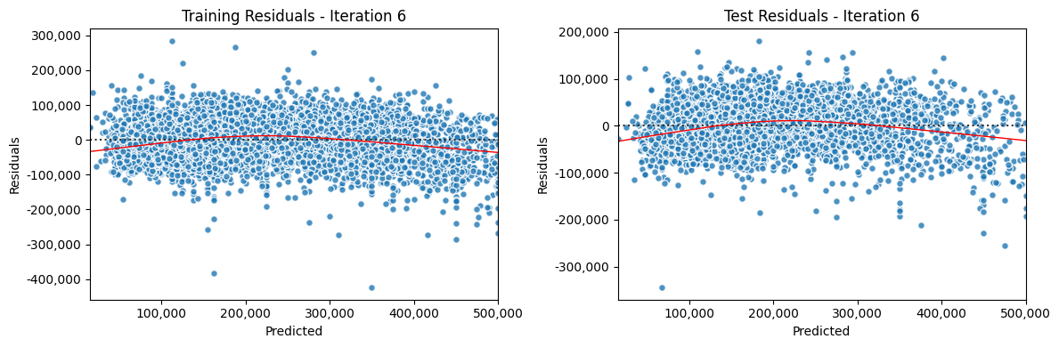
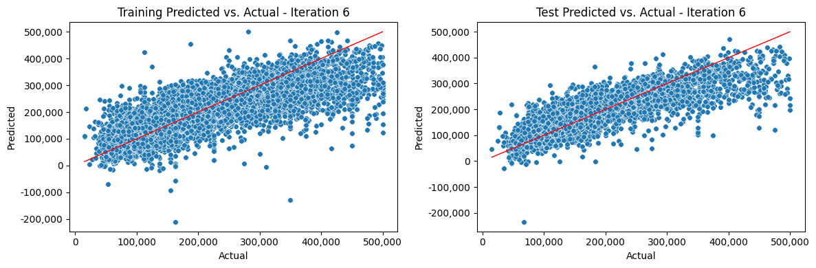
Coefficients:
Feature Coefficient
1 ocean_proximity_<1H OCEAN 13,653.03
2 ocean_proximity_INLAND -19,527.72
3 ocean_proximity_ISLAND 100.12
4 ocean_proximity_NEAR BAY -5,699.28
5 ocean_proximity_NEAR OCEAN 15,294.44
6 total_rooms_log -49,206.07
7 total_bedrooms_log 82,928.70
8 population_log -73,367.99
9 households_log 46,297.94
10 median_income 0.30
11 median_income^2 0.00
12 median_income^3 0.00
13 longitude -26,119.29
14 latitude -24,332.90
15 housing_median_age 753.07
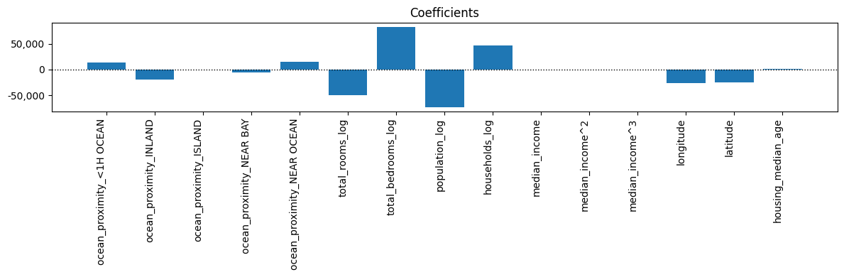
[99]:
# Review the pipeline
iteration_6
[99]:
Pipeline(steps=[('ohe_log_poly3',
ColumnTransformer(force_int_remainder_cols=False,
remainder='passthrough',
transformers=[('ohe',
OneHotEncoder(drop='if_binary',
handle_unknown='ignore'),
['ocean_proximity']),
('log', LogTransformer(),
['total_rooms',
'total_bedrooms',
'population',
'households']),
('poly3',
PolynomialFeatures(degree=3,
include_bias=False),
['median_income'])])),
('linreg', LinearRegression())])In a Jupyter environment, please rerun this cell to show the HTML representation or trust the notebook. On GitHub, the HTML representation is unable to render, please try loading this page with nbviewer.org.
Pipeline(steps=[('ohe_log_poly3',
ColumnTransformer(force_int_remainder_cols=False,
remainder='passthrough',
transformers=[('ohe',
OneHotEncoder(drop='if_binary',
handle_unknown='ignore'),
['ocean_proximity']),
('log', LogTransformer(),
['total_rooms',
'total_bedrooms',
'population',
'households']),
('poly3',
PolynomialFeatures(degree=3,
include_bias=False),
['median_income'])])),
('linreg', LinearRegression())])ColumnTransformer(force_int_remainder_cols=False, remainder='passthrough',
transformers=[('ohe',
OneHotEncoder(drop='if_binary',
handle_unknown='ignore'),
['ocean_proximity']),
('log', LogTransformer(),
['total_rooms', 'total_bedrooms', 'population',
'households']),
('poly3',
PolynomialFeatures(degree=3,
include_bias=False),
['median_income'])])['ocean_proximity']
OneHotEncoder(drop='if_binary', handle_unknown='ignore')
['total_rooms', 'total_bedrooms', 'population', 'households']
LogTransformer()
['median_income']
PolynomialFeatures(degree=3, include_bias=False)
['longitude', 'latitude', 'housing_median_age']
passthrough
LinearRegression()
Iteration 7: Linear Regression with OHE, Log#
[100]:
# The Polynomials aren't having much of an effect, their coefficients are almost 0.
# Let's try one-hot encoding without the polynomial, we didn't try this yet
results_df, iteration_7 = dw.iterate_model(X2_train, X2_test, y2_train, y2_test,
transformers=['ohe', 'log'], model='linreg',
iteration='7', note='X2. Test size: 0.25, Pipeline: OHE > Log > LinReg',
plot=True, lowess=True, coef=True, perm=True, vif=True, decimal=2,
save=True, save_df=results_df, config=my_config)
ITERATION 7 RESULTS
Pipeline: ohe_log -> linreg
Note: X2. Test size: 0.25, Pipeline: OHE > Log > LinReg
May 30, 2024 09:17 AM UTC
Predictions:
Train Test
MSE: 3,237,365,967.08 3,249,712,162.27
RMSE: 56,897.86 57,006.25
MAE: 41,453.54 41,585.27
R^2 Score: 0.64 0.66
Permutation Feature Importance:
Feature Importance Mean Importance Std
median_income 0.94 0.01
total_bedrooms 0.79 0.01
population 0.59 0.01
latitude 0.59 0.01
longitude 0.57 0.01
total_rooms 0.30 0.01
households 0.22 0.00
ocean_proximity 0.06 0.00
housing_median_age 0.02 0.00
Variance Inflation Factor:
Features VIF Multicollinearity
total_bedrooms 32.40 High
households 30.01 High
total_rooms 13.80 High
latitude 8.74 Moderate
longitude 8.43 Moderate
population 6.75 Moderate
median_income 1.83 Low
housing_median_age 1.30 Low
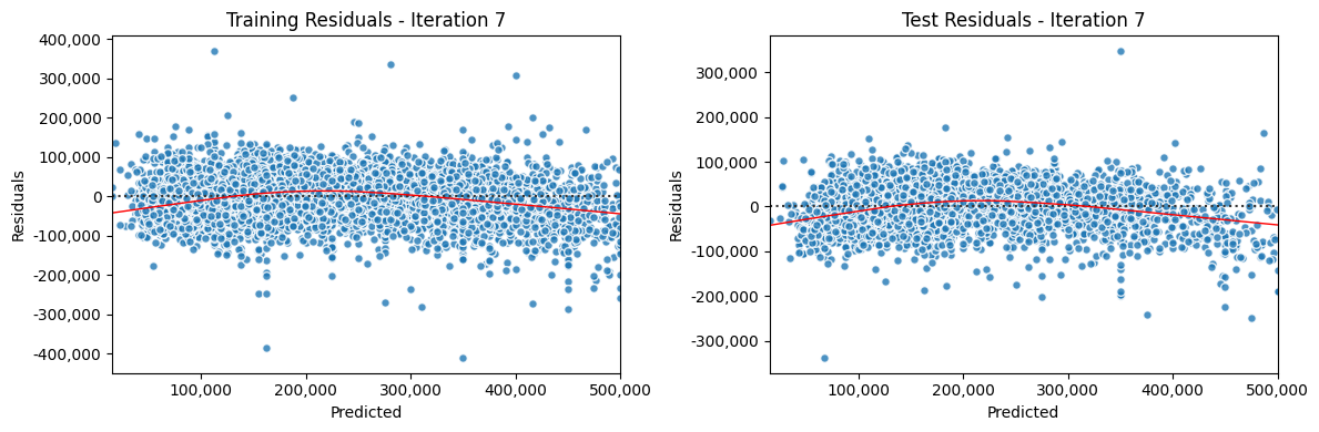
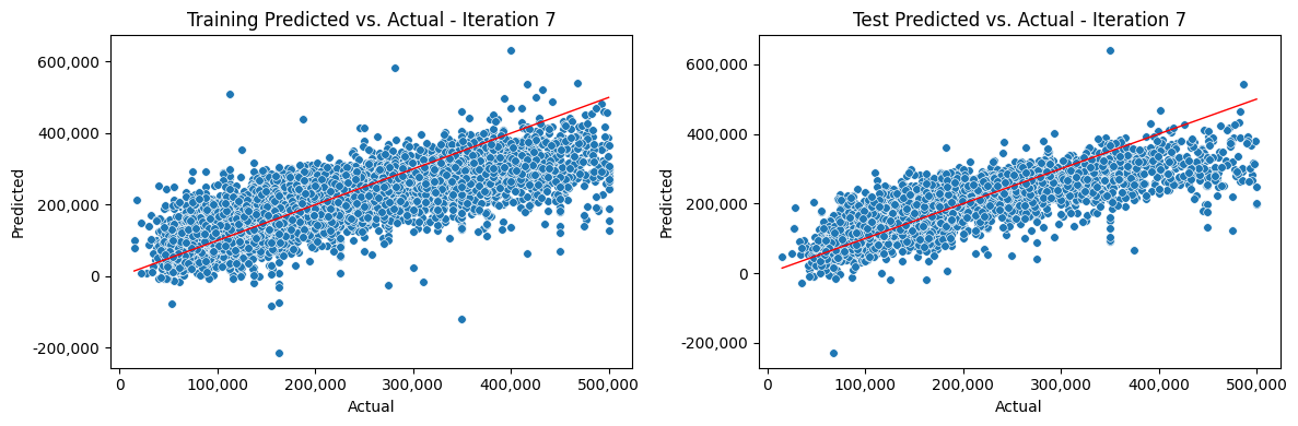
Coefficients:
Feature Coefficient
1 ocean_proximity_<1H OCEAN -4,563.40
2 ocean_proximity_INLAND -37,995.49
3 ocean_proximity_ISLAND 68,751.51
4 ocean_proximity_NEAR BAY -23,027.74
5 ocean_proximity_NEAR OCEAN -3,164.88
6 total_rooms_log -50,498.18
7 total_bedrooms_log 84,183.78
8 population_log -71,995.45
9 households_log 44,404.94
10 longitude -25,874.39
11 latitude -24,114.88
12 housing_median_age 728.72
13 median_income 4.17
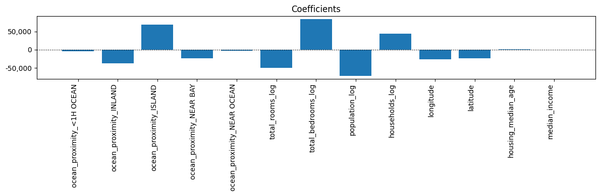
[101]:
# Review the pipeline
iteration_7
[101]:
Pipeline(steps=[('ohe_log',
ColumnTransformer(force_int_remainder_cols=False,
remainder='passthrough',
transformers=[('ohe',
OneHotEncoder(drop='if_binary',
handle_unknown='ignore'),
['ocean_proximity']),
('log', LogTransformer(),
['total_rooms',
'total_bedrooms',
'population',
'households'])])),
('linreg', LinearRegression())])In a Jupyter environment, please rerun this cell to show the HTML representation or trust the notebook. On GitHub, the HTML representation is unable to render, please try loading this page with nbviewer.org.
Pipeline(steps=[('ohe_log',
ColumnTransformer(force_int_remainder_cols=False,
remainder='passthrough',
transformers=[('ohe',
OneHotEncoder(drop='if_binary',
handle_unknown='ignore'),
['ocean_proximity']),
('log', LogTransformer(),
['total_rooms',
'total_bedrooms',
'population',
'households'])])),
('linreg', LinearRegression())])ColumnTransformer(force_int_remainder_cols=False, remainder='passthrough',
transformers=[('ohe',
OneHotEncoder(drop='if_binary',
handle_unknown='ignore'),
['ocean_proximity']),
('log', LogTransformer(),
['total_rooms', 'total_bedrooms', 'population',
'households'])])['ocean_proximity']
OneHotEncoder(drop='if_binary', handle_unknown='ignore')
['total_rooms', 'total_bedrooms', 'population', 'households']
LogTransformer()
['longitude', 'latitude', 'housing_median_age', 'median_income']
passthrough
LinearRegression()
Iteration 8: Ridge with Log, Poly3, Standard and CV#
[102]:
# For illustration, let's try doing a ridge model, and show cross-validation
# We can also turn off VIF and PFI
results_df, iteration_8 = dw.iterate_model(X1_train, X1_test, y1_train, y1_test,
transformers=['log', 'poly3'], scaler='stand', model='ridge', cross=True, cv_folds=5,
iteration='8', note='X1. Test size: 0.25, Pipeline: Log > Poly3 > Stand > Ridge. CV: 5',
plot=True, lowess=True, coef=True, perm=False, vif=False, decimal=2,
save=True, save_df=results_df, config=my_config)
ITERATION 8 RESULTS
Pipeline: log_poly3 -> stand -> ridge
Note: X1. Test size: 0.25, Pipeline: Log > Poly3 > Stand > Ridge. CV: 5
May 30, 2024 09:17 AM UTC
Cross Validation:
Cross-Validation (R^2) Scores for 5 Folds:
Fold 1: 0.63
Fold 2: 0.64
Fold 3: 0.63
Fold 4: 0.63
Fold 5: 0.65
Average: 0.64
Standard Deviation: 0.00
Predictions:
Train Test
MSE: 3,288,332,850.84 3,283,356,079.58
RMSE: 57,343.99 57,300.58
MAE: 42,229.62 42,182.13
R^2 Score: 0.64 0.65


Coefficients:
Feature Coefficient
1 total_rooms_log -45,381.84
2 total_bedrooms_log 69,517.14
3 population_log -53,158.41
4 households_log 31,694.94
5 median_income 11,180.16
6 median_income^2 108,382.39
7 median_income^3 -54,775.23
8 longitude -73,239.73
9 latitude -79,178.20
10 housing_median_age 9,489.76

[103]:
# Review the pipeline
iteration_8
[103]:
Pipeline(steps=[('log_poly3',
ColumnTransformer(force_int_remainder_cols=False,
remainder='passthrough',
transformers=[('log', LogTransformer(),
['total_rooms',
'total_bedrooms',
'population',
'households']),
('poly3',
PolynomialFeatures(degree=3,
include_bias=False),
['median_income'])])),
('stand', StandardScaler()), ('ridge', Ridge())])In a Jupyter environment, please rerun this cell to show the HTML representation or trust the notebook. On GitHub, the HTML representation is unable to render, please try loading this page with nbviewer.org.
Pipeline(steps=[('log_poly3',
ColumnTransformer(force_int_remainder_cols=False,
remainder='passthrough',
transformers=[('log', LogTransformer(),
['total_rooms',
'total_bedrooms',
'population',
'households']),
('poly3',
PolynomialFeatures(degree=3,
include_bias=False),
['median_income'])])),
('stand', StandardScaler()), ('ridge', Ridge())])ColumnTransformer(force_int_remainder_cols=False, remainder='passthrough',
transformers=[('log', LogTransformer(),
['total_rooms', 'total_bedrooms', 'population',
'households']),
('poly3',
PolynomialFeatures(degree=3,
include_bias=False),
['median_income'])])['total_rooms', 'total_bedrooms', 'population', 'households']
LogTransformer()
['median_income']
PolynomialFeatures(degree=3, include_bias=False)
['longitude', 'latitude', 'housing_median_age']
passthrough
StandardScaler()
Ridge()
Iteration 9: Ridge with Log, Poly3, Standard and Grid CV#
[104]:
# Instead of just the cross-validation, let's try a grid search of Ridge hyper-parameters
results_df, iteration_9, grid_9 = dw.iterate_model(X1_train, X1_test, y1_train, y1_test,
transformers=['log', 'poly3'], scaler='stand', model='ridge',
grid=True, grid_params='ridge', grid_cv='kfold_5', grid_verbose=4,
iteration='9', note='X1. Test size: 0.25, Pipeline: Log > Poly3 > Stand > Ridge. Grid CV: 5',
plot=True, lowess=True, coef=True, perm=True, vif=True, decimal=2,
save=True, save_df=results_df, config=my_config)
ITERATION 9 RESULTS
Pipeline: log_poly3 -> stand -> ridge
Note: X1. Test size: 0.25, Pipeline: Log > Poly3 > Stand > Ridge. Grid CV: 5
May 30, 2024 09:17 AM UTC
Grid Search:
Fitting 5 folds for each of 8 candidates, totalling 40 fits
[CV 1/5] END ................ridge__alpha=0.001;, score=0.640 total time= 0.0s
[CV 2/5] END ................ridge__alpha=0.001;, score=0.615 total time= 0.0s
[CV 3/5] END ................ridge__alpha=0.001;, score=0.640 total time= 0.0s
[CV 4/5] END ................ridge__alpha=0.001;, score=0.642 total time= 0.0s
[CV 5/5] END ................ridge__alpha=0.001;, score=0.648 total time= 0.0s
[CV 1/5] END ..................ridge__alpha=0.1;, score=0.640 total time= 0.0s
[CV 2/5] END ..................ridge__alpha=0.1;, score=0.615 total time= 0.0s
[CV 3/5] END ..................ridge__alpha=0.1;, score=0.640 total time= 0.0s
[CV 4/5] END ..................ridge__alpha=0.1;, score=0.642 total time= 0.0s
[CV 5/5] END ..................ridge__alpha=0.1;, score=0.648 total time= 0.0s
[CV 1/5] END ..................ridge__alpha=1.0;, score=0.640 total time= 0.0s
[CV 2/5] END ..................ridge__alpha=1.0;, score=0.615 total time= 0.0s
[CV 3/5] END ..................ridge__alpha=1.0;, score=0.640 total time= 0.0s
[CV 4/5] END ..................ridge__alpha=1.0;, score=0.642 total time= 0.0s
[CV 5/5] END ..................ridge__alpha=1.0;, score=0.648 total time= 0.0s
[CV 1/5] END .................ridge__alpha=10.0;, score=0.640 total time= 0.0s
[CV 2/5] END .................ridge__alpha=10.0;, score=0.615 total time= 0.0s
[CV 3/5] END .................ridge__alpha=10.0;, score=0.640 total time= 0.0s
[CV 4/5] END .................ridge__alpha=10.0;, score=0.642 total time= 0.0s
[CV 5/5] END .................ridge__alpha=10.0;, score=0.646 total time= 0.0s
[CV 1/5] END ................ridge__alpha=100.0;, score=0.636 total time= 0.0s
[CV 2/5] END ................ridge__alpha=100.0;, score=0.614 total time= 0.1s
[CV 3/5] END ................ridge__alpha=100.0;, score=0.636 total time= 0.0s
[CV 4/5] END ................ridge__alpha=100.0;, score=0.638 total time= 0.0s
[CV 5/5] END ................ridge__alpha=100.0;, score=0.639 total time= 0.0s
[CV 1/5] END ...............ridge__alpha=1000.0;, score=0.580 total time= 0.0s
[CV 2/5] END ...............ridge__alpha=1000.0;, score=0.563 total time= 0.0s
[CV 3/5] END ...............ridge__alpha=1000.0;, score=0.582 total time= 0.0s
[CV 4/5] END ...............ridge__alpha=1000.0;, score=0.581 total time= 0.0s
[CV 5/5] END ...............ridge__alpha=1000.0;, score=0.581 total time= 0.0s
[CV 1/5] END ..............ridge__alpha=10000.0;, score=0.438 total time= 0.0s
[CV 2/5] END ..............ridge__alpha=10000.0;, score=0.422 total time= 0.0s
[CV 3/5] END ..............ridge__alpha=10000.0;, score=0.439 total time= 0.0s
[CV 4/5] END ..............ridge__alpha=10000.0;, score=0.435 total time= 0.0s
[CV 5/5] END ..............ridge__alpha=10000.0;, score=0.447 total time= 0.0s
[CV 1/5] END .............ridge__alpha=100000.0;, score=0.180 total time= 0.0s
[CV 2/5] END .............ridge__alpha=100000.0;, score=0.173 total time= 0.0s
[CV 3/5] END .............ridge__alpha=100000.0;, score=0.177 total time= 0.0s
[CV 4/5] END .............ridge__alpha=100000.0;, score=0.181 total time= 0.0s
[CV 5/5] END .............ridge__alpha=100000.0;, score=0.196 total time= 0.0s
Best Grid mean score (r2): 0.64
Best Grid parameters: ridge__alpha: 1.0
Predictions:
Train Test
MSE: 3,288,332,850.84 3,283,356,079.58
RMSE: 57,343.99 57,300.58
MAE: 42,229.62 42,182.13
R^2 Score: 0.64 0.65
Permutation Feature Importance:
Feature Importance Mean Importance Std
latitude 1.38 0.01
longitude 1.17 0.01
total_bedrooms 1.06 0.01
median_income 1.04 0.01
population 0.62 0.01
total_rooms 0.46 0.01
households 0.22 0.00
housing_median_age 0.02 0.00
Variance Inflation Factor:
Features VIF Multicollinearity
total_bedrooms 32.40 High
households 30.01 High
total_rooms 13.80 High
latitude 8.74 Moderate
longitude 8.43 Moderate
population 6.75 Moderate
median_income 1.83 Low
housing_median_age 1.30 Low
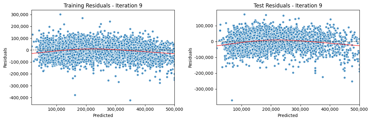
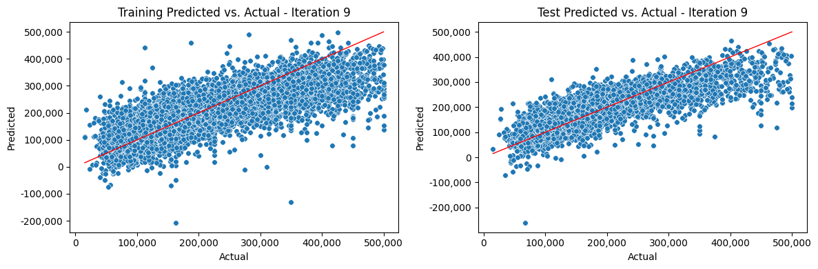
Coefficients:
Feature Coefficient
1 total_rooms_log -45,381.84
2 total_bedrooms_log 69,517.14
3 population_log -53,158.41
4 households_log 31,694.94
5 median_income 11,180.16
6 median_income^2 108,382.39
7 median_income^3 -54,775.23
8 longitude -73,239.73
9 latitude -79,178.20
10 housing_median_age 9,489.76
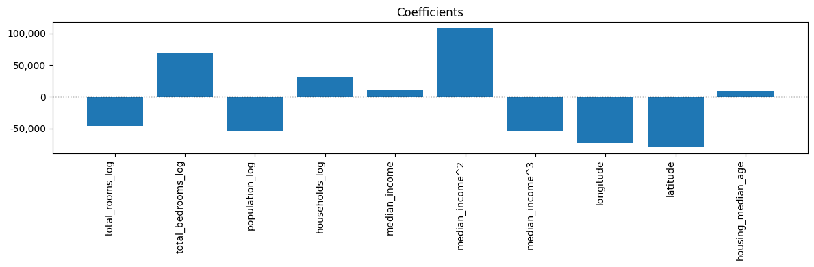
[105]:
# Review the pipeline
iteration_9
[105]:
GridSearchCV(cv=KFold(n_splits=5, random_state=42, shuffle=True),
estimator=Pipeline(steps=[('log_poly3',
ColumnTransformer(force_int_remainder_cols=False,
remainder='passthrough',
transformers=[('log',
LogTransformer(),
['total_rooms',
'total_bedrooms',
'population',
'households']),
('poly3',
PolynomialFeatures(degree=3,
include_bias=False),
['median_income'])])),
('stand', StandardScaler()),
('ridge', Ridge())]),
param_grid={'ridge__alpha': array([1.e-03, 1.e-01, 1.e+00, 1.e+01, 1.e+02, 1.e+03, 1.e+04, 1.e+05])},
scoring='r2', verbose=4)In a Jupyter environment, please rerun this cell to show the HTML representation or trust the notebook. On GitHub, the HTML representation is unable to render, please try loading this page with nbviewer.org.
GridSearchCV(cv=KFold(n_splits=5, random_state=42, shuffle=True),
estimator=Pipeline(steps=[('log_poly3',
ColumnTransformer(force_int_remainder_cols=False,
remainder='passthrough',
transformers=[('log',
LogTransformer(),
['total_rooms',
'total_bedrooms',
'population',
'households']),
('poly3',
PolynomialFeatures(degree=3,
include_bias=False),
['median_income'])])),
('stand', StandardScaler()),
('ridge', Ridge())]),
param_grid={'ridge__alpha': array([1.e-03, 1.e-01, 1.e+00, 1.e+01, 1.e+02, 1.e+03, 1.e+04, 1.e+05])},
scoring='r2', verbose=4)Pipeline(steps=[('log_poly3',
ColumnTransformer(force_int_remainder_cols=False,
remainder='passthrough',
transformers=[('log', LogTransformer(),
['total_rooms',
'total_bedrooms',
'population',
'households']),
('poly3',
PolynomialFeatures(degree=3,
include_bias=False),
['median_income'])])),
('stand', StandardScaler()), ('ridge', Ridge())])ColumnTransformer(force_int_remainder_cols=False, remainder='passthrough',
transformers=[('log', LogTransformer(),
['total_rooms', 'total_bedrooms', 'population',
'households']),
('poly3',
PolynomialFeatures(degree=3,
include_bias=False),
['median_income'])])['total_rooms', 'total_bedrooms', 'population', 'households']
LogTransformer()
['median_income']
PolynomialFeatures(degree=3, include_bias=False)
['longitude', 'latitude', 'housing_median_age']
passthrough
StandardScaler()
Ridge()
Iteration 10: Decision Tree and Random Grid CV#
[106]:
# Let's try a Decision Tree and do a Random Grid Search over a few hyper-parameters
results_df, iteration_10, grid_10 = dw.iterate_model(X1_train, X1_test, y1_train, y1_test,
model='tree_reg',
grid=True, search_type='random', grid_params='tree_reg', grid_cv='kfold_5', grid_verbose=4,
iteration='10', note='X1. Test size: 0.25, Pipeline: Tree. Random Grid CV: 5',
plot=True, lowess=True, coef=True, perm=True, vif=True, decimal=2,
save=True, save_df=results_df, config=my_config)
ITERATION 10 RESULTS
Pipeline: tree_reg
Note: X1. Test size: 0.25, Pipeline: Tree. Random Grid CV: 5
May 30, 2024 09:17 AM UTC
Randomized Grid Search:
Fitting 5 folds for each of 10 candidates, totalling 50 fits
[CV 1/5] END tree_reg__criterion=squared_error, tree_reg__max_depth=7, tree_reg__min_samples_leaf=4, tree_reg__min_samples_split=15;, score=0.620 total time= 0.1s
[CV 2/5] END tree_reg__criterion=squared_error, tree_reg__max_depth=7, tree_reg__min_samples_leaf=4, tree_reg__min_samples_split=15;, score=0.614 total time= 0.0s
[CV 3/5] END tree_reg__criterion=squared_error, tree_reg__max_depth=7, tree_reg__min_samples_leaf=4, tree_reg__min_samples_split=15;, score=0.649 total time= 0.0s
[CV 4/5] END tree_reg__criterion=squared_error, tree_reg__max_depth=7, tree_reg__min_samples_leaf=4, tree_reg__min_samples_split=15;, score=0.658 total time= 0.0s
[CV 5/5] END tree_reg__criterion=squared_error, tree_reg__max_depth=7, tree_reg__min_samples_leaf=4, tree_reg__min_samples_split=15;, score=0.656 total time= 0.0s
[CV 1/5] END tree_reg__criterion=poisson, tree_reg__max_depth=5, tree_reg__min_samples_leaf=2, tree_reg__min_samples_split=10;, score=0.539 total time= 0.0s
[CV 2/5] END tree_reg__criterion=poisson, tree_reg__max_depth=5, tree_reg__min_samples_leaf=2, tree_reg__min_samples_split=10;, score=0.528 total time= 0.0s
[CV 3/5] END tree_reg__criterion=poisson, tree_reg__max_depth=5, tree_reg__min_samples_leaf=2, tree_reg__min_samples_split=10;, score=0.541 total time= 0.0s
[CV 4/5] END tree_reg__criterion=poisson, tree_reg__max_depth=5, tree_reg__min_samples_leaf=2, tree_reg__min_samples_split=10;, score=0.550 total time= 0.0s
[CV 5/5] END tree_reg__criterion=poisson, tree_reg__max_depth=5, tree_reg__min_samples_leaf=2, tree_reg__min_samples_split=10;, score=0.566 total time= 0.0s
[CV 1/5] END tree_reg__criterion=poisson, tree_reg__max_depth=3, tree_reg__min_samples_leaf=4, tree_reg__min_samples_split=10;, score=0.448 total time= 0.0s
[CV 2/5] END tree_reg__criterion=poisson, tree_reg__max_depth=3, tree_reg__min_samples_leaf=4, tree_reg__min_samples_split=10;, score=0.427 total time= 0.0s
[CV 3/5] END tree_reg__criterion=poisson, tree_reg__max_depth=3, tree_reg__min_samples_leaf=4, tree_reg__min_samples_split=10;, score=0.456 total time= 0.0s
[CV 4/5] END tree_reg__criterion=poisson, tree_reg__max_depth=3, tree_reg__min_samples_leaf=4, tree_reg__min_samples_split=10;, score=0.463 total time= 0.0s
[CV 5/5] END tree_reg__criterion=poisson, tree_reg__max_depth=3, tree_reg__min_samples_leaf=4, tree_reg__min_samples_split=10;, score=0.474 total time= 0.0s
[CV 1/5] END tree_reg__criterion=absolute_error, tree_reg__max_depth=3, tree_reg__min_samples_leaf=2, tree_reg__min_samples_split=15;, score=0.426 total time= 2.9s
[CV 2/5] END tree_reg__criterion=absolute_error, tree_reg__max_depth=3, tree_reg__min_samples_leaf=2, tree_reg__min_samples_split=15;, score=0.396 total time= 2.8s
[CV 3/5] END tree_reg__criterion=absolute_error, tree_reg__max_depth=3, tree_reg__min_samples_leaf=2, tree_reg__min_samples_split=15;, score=0.416 total time= 3.0s
[CV 4/5] END tree_reg__criterion=absolute_error, tree_reg__max_depth=3, tree_reg__min_samples_leaf=2, tree_reg__min_samples_split=15;, score=0.426 total time= 3.0s
[CV 5/5] END tree_reg__criterion=absolute_error, tree_reg__max_depth=3, tree_reg__min_samples_leaf=2, tree_reg__min_samples_split=15;, score=0.460 total time= 3.0s
[CV 1/5] END tree_reg__criterion=squared_error, tree_reg__max_depth=3, tree_reg__min_samples_leaf=6, tree_reg__min_samples_split=15;, score=0.446 total time= 0.0s
[CV 2/5] END tree_reg__criterion=squared_error, tree_reg__max_depth=3, tree_reg__min_samples_leaf=6, tree_reg__min_samples_split=15;, score=0.428 total time= 0.0s
[CV 3/5] END tree_reg__criterion=squared_error, tree_reg__max_depth=3, tree_reg__min_samples_leaf=6, tree_reg__min_samples_split=15;, score=0.453 total time= 0.0s
[CV 4/5] END tree_reg__criterion=squared_error, tree_reg__max_depth=3, tree_reg__min_samples_leaf=6, tree_reg__min_samples_split=15;, score=0.446 total time= 0.0s
[CV 5/5] END tree_reg__criterion=squared_error, tree_reg__max_depth=3, tree_reg__min_samples_leaf=6, tree_reg__min_samples_split=15;, score=0.474 total time= 0.0s
[CV 1/5] END tree_reg__criterion=squared_error, tree_reg__max_depth=5, tree_reg__min_samples_leaf=4, tree_reg__min_samples_split=10;, score=0.534 total time= 0.0s
[CV 2/5] END tree_reg__criterion=squared_error, tree_reg__max_depth=5, tree_reg__min_samples_leaf=4, tree_reg__min_samples_split=10;, score=0.529 total time= 0.0s
[CV 3/5] END tree_reg__criterion=squared_error, tree_reg__max_depth=5, tree_reg__min_samples_leaf=4, tree_reg__min_samples_split=10;, score=0.551 total time= 0.0s
[CV 4/5] END tree_reg__criterion=squared_error, tree_reg__max_depth=5, tree_reg__min_samples_leaf=4, tree_reg__min_samples_split=10;, score=0.555 total time= 0.0s
[CV 5/5] END tree_reg__criterion=squared_error, tree_reg__max_depth=5, tree_reg__min_samples_leaf=4, tree_reg__min_samples_split=10;, score=0.576 total time= 0.0s
[CV 1/5] END tree_reg__criterion=friedman_mse, tree_reg__max_depth=3, tree_reg__min_samples_leaf=4, tree_reg__min_samples_split=5;, score=0.446 total time= 0.0s
[CV 2/5] END tree_reg__criterion=friedman_mse, tree_reg__max_depth=3, tree_reg__min_samples_leaf=4, tree_reg__min_samples_split=5;, score=0.428 total time= 0.0s
[CV 3/5] END tree_reg__criterion=friedman_mse, tree_reg__max_depth=3, tree_reg__min_samples_leaf=4, tree_reg__min_samples_split=5;, score=0.453 total time= 0.0s
[CV 4/5] END tree_reg__criterion=friedman_mse, tree_reg__max_depth=3, tree_reg__min_samples_leaf=4, tree_reg__min_samples_split=5;, score=0.446 total time= 0.0s
[CV 5/5] END tree_reg__criterion=friedman_mse, tree_reg__max_depth=3, tree_reg__min_samples_leaf=4, tree_reg__min_samples_split=5;, score=0.474 total time= 0.0s
[CV 1/5] END tree_reg__criterion=friedman_mse, tree_reg__max_depth=7, tree_reg__min_samples_leaf=2, tree_reg__min_samples_split=5;, score=0.621 total time= 0.1s
[CV 2/5] END tree_reg__criterion=friedman_mse, tree_reg__max_depth=7, tree_reg__min_samples_leaf=2, tree_reg__min_samples_split=5;, score=0.613 total time= 0.1s
[CV 3/5] END tree_reg__criterion=friedman_mse, tree_reg__max_depth=7, tree_reg__min_samples_leaf=2, tree_reg__min_samples_split=5;, score=0.647 total time= 0.1s
[CV 4/5] END tree_reg__criterion=friedman_mse, tree_reg__max_depth=7, tree_reg__min_samples_leaf=2, tree_reg__min_samples_split=5;, score=0.658 total time= 0.1s
[CV 5/5] END tree_reg__criterion=friedman_mse, tree_reg__max_depth=7, tree_reg__min_samples_leaf=2, tree_reg__min_samples_split=5;, score=0.654 total time= 0.1s
[CV 1/5] END tree_reg__criterion=absolute_error, tree_reg__max_depth=5, tree_reg__min_samples_leaf=4, tree_reg__min_samples_split=15;, score=0.534 total time= 3.4s
[CV 2/5] END tree_reg__criterion=absolute_error, tree_reg__max_depth=5, tree_reg__min_samples_leaf=4, tree_reg__min_samples_split=15;, score=0.484 total time= 3.5s
[CV 3/5] END tree_reg__criterion=absolute_error, tree_reg__max_depth=5, tree_reg__min_samples_leaf=4, tree_reg__min_samples_split=15;, score=0.529 total time= 4.2s
[CV 4/5] END tree_reg__criterion=absolute_error, tree_reg__max_depth=5, tree_reg__min_samples_leaf=4, tree_reg__min_samples_split=15;, score=0.548 total time= 3.6s
[CV 5/5] END tree_reg__criterion=absolute_error, tree_reg__max_depth=5, tree_reg__min_samples_leaf=4, tree_reg__min_samples_split=15;, score=0.568 total time= 3.5s
[CV 1/5] END tree_reg__criterion=poisson, tree_reg__max_depth=5, tree_reg__min_samples_leaf=2, tree_reg__min_samples_split=15;, score=0.539 total time= 0.0s
[CV 2/5] END tree_reg__criterion=poisson, tree_reg__max_depth=5, tree_reg__min_samples_leaf=2, tree_reg__min_samples_split=15;, score=0.528 total time= 0.0s
[CV 3/5] END tree_reg__criterion=poisson, tree_reg__max_depth=5, tree_reg__min_samples_leaf=2, tree_reg__min_samples_split=15;, score=0.541 total time= 0.0s
[CV 4/5] END tree_reg__criterion=poisson, tree_reg__max_depth=5, tree_reg__min_samples_leaf=2, tree_reg__min_samples_split=15;, score=0.550 total time= 0.0s
[CV 5/5] END tree_reg__criterion=poisson, tree_reg__max_depth=5, tree_reg__min_samples_leaf=2, tree_reg__min_samples_split=15;, score=0.566 total time= 0.0s
Best Grid mean score (r2): 0.64
Best Grid parameters: tree_reg__min_samples_split: 15, tree_reg__min_samples_leaf: 4, tree_reg__max_depth: 7, tree_reg__criterion: squared_error
Predictions:
Train Test
MSE: 2,944,707,111.06 3,340,337,711.85
RMSE: 54,265.16 57,795.65
MAE: 39,005.07 41,031.86
R^2 Score: 0.68 0.65
Permutation Feature Importance:
Feature Importance Mean Importance Std
latitude 0.92 0.01
longitude 0.81 0.01
median_income 0.79 0.01
housing_median_age 0.07 0.00
total_bedrooms 0.03 0.00
population 0.01 0.00
total_rooms 0.01 0.00
households 0.00 0.00
Variance Inflation Factor:
Features VIF Multicollinearity
total_bedrooms 32.40 High
households 30.01 High
total_rooms 13.80 High
latitude 8.74 Moderate
longitude 8.43 Moderate
population 6.75 Moderate
median_income 1.83 Low
housing_median_age 1.30 Low
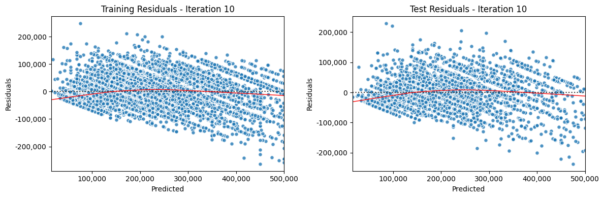
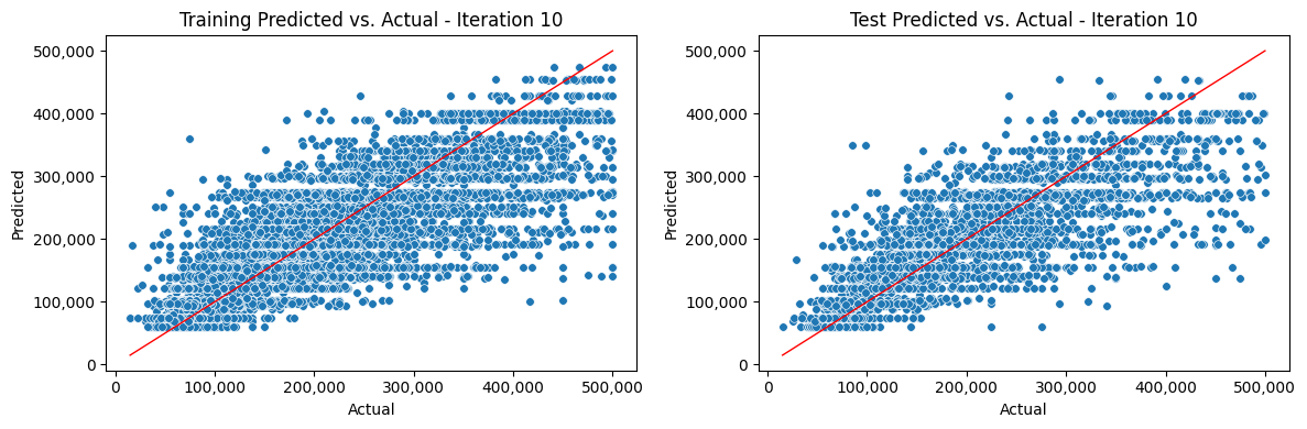
[107]:
# Review the pipeline
iteration_10
[107]:
RandomizedSearchCV(cv=KFold(n_splits=5, random_state=42, shuffle=True),
estimator=Pipeline(steps=[('tree_reg',
DecisionTreeRegressor(random_state=42))]),
param_distributions={'tree_reg__criterion': ['poisson',
'friedman_mse',
'squared_error',
'absolute_error'],
'tree_reg__max_depth': [3, 5, 7],
'tree_reg__min_samples_leaf': [2, 4, 6],
'tree_reg__min_samples_split': [5, 10,
15]},
random_state=42, scoring='r2', verbose=4)In a Jupyter environment, please rerun this cell to show the HTML representation or trust the notebook. On GitHub, the HTML representation is unable to render, please try loading this page with nbviewer.org.
RandomizedSearchCV(cv=KFold(n_splits=5, random_state=42, shuffle=True),
estimator=Pipeline(steps=[('tree_reg',
DecisionTreeRegressor(random_state=42))]),
param_distributions={'tree_reg__criterion': ['poisson',
'friedman_mse',
'squared_error',
'absolute_error'],
'tree_reg__max_depth': [3, 5, 7],
'tree_reg__min_samples_leaf': [2, 4, 6],
'tree_reg__min_samples_split': [5, 10,
15]},
random_state=42, scoring='r2', verbose=4)Pipeline(steps=[('tree_reg',
DecisionTreeRegressor(max_depth=7, min_samples_leaf=4,
min_samples_split=15,
random_state=42))])DecisionTreeRegressor(max_depth=7, min_samples_leaf=4, min_samples_split=15,
random_state=42)[108]:
# Review the grid parameters
iteration_10.get_params()
[108]:
{'cv': KFold(n_splits=5, random_state=42, shuffle=True),
'error_score': nan,
'estimator__memory': None,
'estimator__steps': [('tree_reg', DecisionTreeRegressor(random_state=42))],
'estimator__verbose': False,
'estimator__tree_reg': DecisionTreeRegressor(random_state=42),
'estimator__tree_reg__ccp_alpha': 0.0,
'estimator__tree_reg__criterion': 'squared_error',
'estimator__tree_reg__max_depth': None,
'estimator__tree_reg__max_features': None,
'estimator__tree_reg__max_leaf_nodes': None,
'estimator__tree_reg__min_impurity_decrease': 0.0,
'estimator__tree_reg__min_samples_leaf': 1,
'estimator__tree_reg__min_samples_split': 2,
'estimator__tree_reg__min_weight_fraction_leaf': 0.0,
'estimator__tree_reg__monotonic_cst': None,
'estimator__tree_reg__random_state': 42,
'estimator__tree_reg__splitter': 'best',
'estimator': Pipeline(steps=[('tree_reg', DecisionTreeRegressor(random_state=42))]),
'n_iter': 10,
'n_jobs': None,
'param_distributions': {'tree_reg__max_depth': [3, 5, 7],
'tree_reg__min_samples_split': [5, 10, 15],
'tree_reg__criterion': ['poisson',
'friedman_mse',
'squared_error',
'absolute_error'],
'tree_reg__min_samples_leaf': [2, 4, 6]},
'pre_dispatch': '2*n_jobs',
'random_state': 42,
'refit': True,
'return_train_score': False,
'scoring': 'r2',
'verbose': 4}
Review the Results#
Now that we’ve explored a few iterations, let’s compare the results. We’ll use dw.format_df to make the numbers easier to read. If we didn’t use this, we’d see a lot of scientific notation and long decimal places that are unnecessary.
[109]:
# Review the results, formatted for better readability
formatted_results_df = dw.format_df(results_df, large_num_cols=['Train MSE', 'Test MSE', 'Train RMSE', 'Test RMSE',
'Train MAE', 'Test MAE'], small_num_cols=['Train R^2 Score', 'Test R^2 Score', 'Best Grid Mean Score'])
formatted_results_df
[109]:
| Iteration | Train MSE | Test MSE | Train RMSE | Test RMSE | Train MAE | Test MAE | Train R^2 Score | Test R^2 Score | Pipeline | Best Grid Params | Note | Date | Best Grid Mean Score | |
|---|---|---|---|---|---|---|---|---|---|---|---|---|---|---|
| 0 | 1 | 3,568,722,087 | 3,614,822,637 | 59,739 | 60,123 | 44,354 | 44,485 | 0.61 | 0.62 | linreg | NaN | X1. Baseline. Test size: 0.25, Pipeline: LinReg | May 30, 2024 09:17 AM UTC | NaN |
| 1 | 2 | 3,333,110,642 | 3,356,136,123 | 57,733 | 57,932 | 42,498 | 42,621 | 0.63 | 0.64 | log -> linreg | NaN | X1. Test size: 0.25, Pipeline: Log > LinReg | May 30, 2024 09:17 AM UTC | NaN |
| 2 | 3 | 3,329,236,889 | 3,350,722,400 | 57,700 | 57,885 | 42,383 | 42,493 | 0.63 | 0.64 | log_poly2 -> linreg | NaN | X1. Test size: 0.25, Pipeline: Log > Poly2 > LinReg | May 30, 2024 09:17 AM UTC | NaN |
| 3 | 4 | 3,231,250,156 | 3,242,416,486 | 56,844 | 56,942 | 41,276 | 41,406 | 0.64 | 0.66 | ohe_log_poly2 -> linreg | NaN | X2. Test size: 0.25, Pipeline: OHE > Log > Poly2 > LinReg | May 30, 2024 09:17 AM UTC | NaN |
| 4 | 5 | 3,323,311,153 | 3,339,547,363 | 57,648 | 57,789 | 42,307 | 42,379 | 0.63 | 0.65 | ord_log_poly2 -> linreg | NaN | X2. Test size: 0.25, Pipeline: Ord > Log > Poly2 > LinReg | May 30, 2024 09:17 AM UTC | NaN |
| 5 | 6 | 3,191,564,997 | 3,179,359,775 | 56,494 | 56,386 | 41,117 | 41,108 | 0.65 | 0.66 | ohe_log_poly3 -> linreg | NaN | X2. Test size: 0.25, Pipeline: OHE > Log > Poly3 > LinReg | May 30, 2024 09:17 AM UTC | NaN |
| 6 | 7 | 3,237,365,967 | 3,249,712,162 | 56,898 | 57,006 | 41,454 | 41,585 | 0.64 | 0.66 | ohe_log -> linreg | NaN | X2. Test size: 0.25, Pipeline: OHE > Log > LinReg | May 30, 2024 09:17 AM UTC | NaN |
| 7 | 8 | 3,288,332,851 | 3,283,356,080 | 57,344 | 57,301 | 42,230 | 42,182 | 0.64 | 0.65 | log_poly3 -> stand -> ridge | NaN | X1. Test size: 0.25, Pipeline: Log > Poly3 > Stand > Ridge. CV: 5 | May 30, 2024 09:17 AM UTC | NaN |
| 8 | 9 | 3,288,332,851 | 3,283,356,080 | 57,344 | 57,301 | 42,230 | 42,182 | 0.64 | 0.65 | log_poly3 -> stand -> ridge | {'ridge__alpha': 1.0} | X1. Test size: 0.25, Pipeline: Log > Poly3 > Stand > Ridge. Grid CV: 5 | May 30, 2024 09:17 AM UTC | 0.64 |
| 9 | 10 | 2,944,707,111 | 3,340,337,712 | 54,265 | 57,796 | 39,005 | 41,032 | 0.68 | 0.65 | tree_reg | {'tree_reg__min_samples_split': 15, 'tree_reg__min_samples_leaf': 4, 'tree_reg__max_depth': 7, 'tree_reg__criterion': 'squared_error'} | X1. Test size: 0.25, Pipeline: Tree. Random Grid CV: 5 | May 30, 2024 09:17 AM UTC | 0.64 |
Plot the Results#
Let’s plot the results so it’s easier to see which model performed the best. We’ll look at ‘Train R^2 Score’ and ‘Test R^2 Score’ across each model ‘Iteration’. And then we’ll look at ‘Train MAE’ and ‘Test MAE’ across each model ‘Iteration’. We’ll use dw.plot_results to simplify this to one line of code, and automatically select the best result, which will be marked on the chart with a vertical line.
[110]:
# Compare train/test R^2 scores across model iterations, and select the best 'Test R^2 Score'
dw.plot_results(results_df, metrics=['Train R^2 Score', 'Test R^2 Score'], y_label='R^2 Score',
select_metric='Test R^2 Score', select_criteria='max', decimal=4)
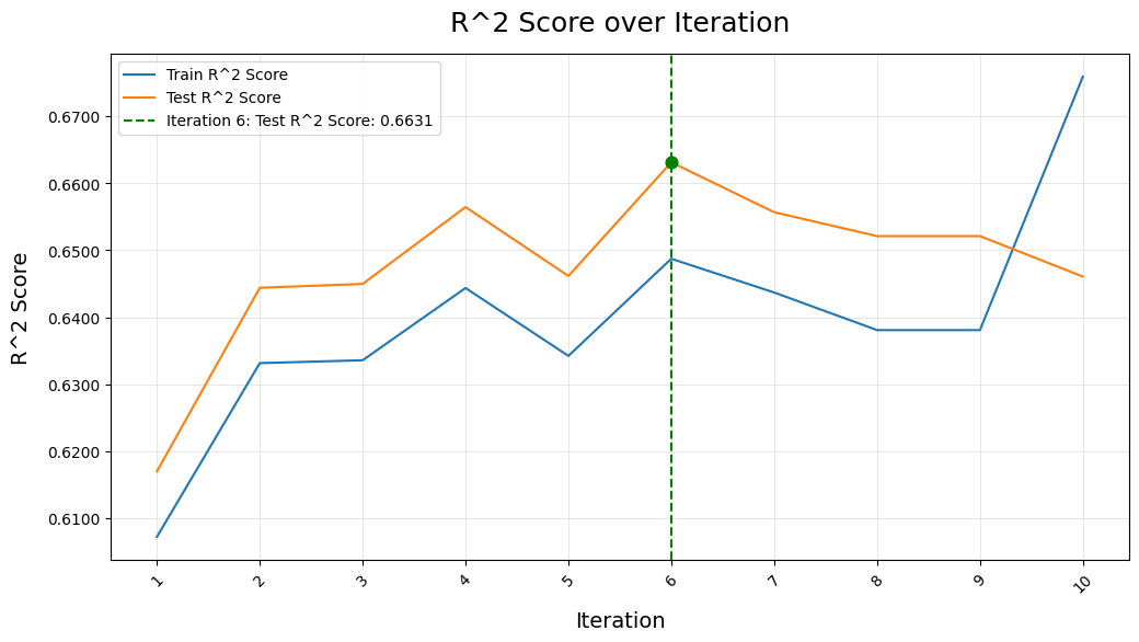
[111]:
# Compare train/test MAE scores across model iterations, and select the best 'Test MAE'
dw.plot_results(results_df, metrics=['Train MAE', 'Test MAE'], y_label='Mean Absolute Error',
select_metric='Test MAE', select_criteria='min', decimal=0)
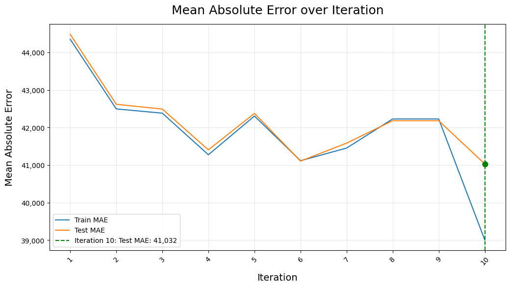
Examine the Final Model#
Iteration 6, a Linear Regression, seems to be the best model. Even though Iteration 10, the Decision Tree, had a lower Test MAE, its Test R^2 Score was lower and overfit on the Train Data. Now that we know the best model, let’s take a look at its details. With every iteration we ran, we saved the fitted model as an object. For example, we entered results_df, iteration_6 = dw.iterate_model(...) which both updated the results_df dataframe by appending the data from iteration 6, and stored
the model as iteration_6.
[112]:
# Review the final model pipeline
iteration_6
[112]:
Pipeline(steps=[('ohe_log_poly3',
ColumnTransformer(force_int_remainder_cols=False,
remainder='passthrough',
transformers=[('ohe',
OneHotEncoder(drop='if_binary',
handle_unknown='ignore'),
['ocean_proximity']),
('log', LogTransformer(),
['total_rooms',
'total_bedrooms',
'population',
'households']),
('poly3',
PolynomialFeatures(degree=3,
include_bias=False),
['median_income'])])),
('linreg', LinearRegression())])In a Jupyter environment, please rerun this cell to show the HTML representation or trust the notebook. On GitHub, the HTML representation is unable to render, please try loading this page with nbviewer.org.
Pipeline(steps=[('ohe_log_poly3',
ColumnTransformer(force_int_remainder_cols=False,
remainder='passthrough',
transformers=[('ohe',
OneHotEncoder(drop='if_binary',
handle_unknown='ignore'),
['ocean_proximity']),
('log', LogTransformer(),
['total_rooms',
'total_bedrooms',
'population',
'households']),
('poly3',
PolynomialFeatures(degree=3,
include_bias=False),
['median_income'])])),
('linreg', LinearRegression())])ColumnTransformer(force_int_remainder_cols=False, remainder='passthrough',
transformers=[('ohe',
OneHotEncoder(drop='if_binary',
handle_unknown='ignore'),
['ocean_proximity']),
('log', LogTransformer(),
['total_rooms', 'total_bedrooms', 'population',
'households']),
('poly3',
PolynomialFeatures(degree=3,
include_bias=False),
['median_income'])])['ocean_proximity']
OneHotEncoder(drop='if_binary', handle_unknown='ignore')
['total_rooms', 'total_bedrooms', 'population', 'households']
LogTransformer()
['median_income']
PolynomialFeatures(degree=3, include_bias=False)
['longitude', 'latitude', 'housing_median_age']
passthrough
LinearRegression()
[113]:
# Review the final pipeline parameters
iteration_6.get_params()
[113]:
{'memory': None,
'steps': [('ohe_log_poly3',
ColumnTransformer(force_int_remainder_cols=False, remainder='passthrough',
transformers=[('ohe',
OneHotEncoder(drop='if_binary',
handle_unknown='ignore'),
['ocean_proximity']),
('log', LogTransformer(),
['total_rooms', 'total_bedrooms', 'population',
'households']),
('poly3',
PolynomialFeatures(degree=3,
include_bias=False),
['median_income'])])),
('linreg', LinearRegression())],
'verbose': False,
'ohe_log_poly3': ColumnTransformer(force_int_remainder_cols=False, remainder='passthrough',
transformers=[('ohe',
OneHotEncoder(drop='if_binary',
handle_unknown='ignore'),
['ocean_proximity']),
('log', LogTransformer(),
['total_rooms', 'total_bedrooms', 'population',
'households']),
('poly3',
PolynomialFeatures(degree=3,
include_bias=False),
['median_income'])]),
'linreg': LinearRegression(),
'ohe_log_poly3__force_int_remainder_cols': False,
'ohe_log_poly3__n_jobs': None,
'ohe_log_poly3__remainder': 'passthrough',
'ohe_log_poly3__sparse_threshold': 0.3,
'ohe_log_poly3__transformer_weights': None,
'ohe_log_poly3__transformers': [('ohe',
OneHotEncoder(drop='if_binary', handle_unknown='ignore'),
['ocean_proximity']),
('log',
LogTransformer(),
['total_rooms', 'total_bedrooms', 'population', 'households']),
('poly3',
PolynomialFeatures(degree=3, include_bias=False),
['median_income'])],
'ohe_log_poly3__verbose': False,
'ohe_log_poly3__verbose_feature_names_out': True,
'ohe_log_poly3__ohe': OneHotEncoder(drop='if_binary', handle_unknown='ignore'),
'ohe_log_poly3__log': LogTransformer(),
'ohe_log_poly3__poly3': PolynomialFeatures(degree=3, include_bias=False),
'ohe_log_poly3__ohe__categories': 'auto',
'ohe_log_poly3__ohe__drop': 'if_binary',
'ohe_log_poly3__ohe__dtype': numpy.float64,
'ohe_log_poly3__ohe__feature_name_combiner': 'concat',
'ohe_log_poly3__ohe__handle_unknown': 'ignore',
'ohe_log_poly3__ohe__max_categories': None,
'ohe_log_poly3__ohe__min_frequency': None,
'ohe_log_poly3__ohe__sparse_output': True,
'ohe_log_poly3__poly3__degree': 3,
'ohe_log_poly3__poly3__include_bias': False,
'ohe_log_poly3__poly3__interaction_only': False,
'ohe_log_poly3__poly3__order': 'C',
'linreg__copy_X': True,
'linreg__fit_intercept': True,
'linreg__n_jobs': None,
'linreg__positive': False}
[114]:
# Note the model coefficients are not part of the pipeline parameters, they are found here:
iteration_6.steps[-1][1].coef_
[114]:
array([[-4.56340164e+03, -3.79954870e+04, 6.87515120e+04,
-2.30277393e+04, -3.16488408e+03, -5.04981768e+04,
8.41837756e+04, -7.19954467e+04, 4.44049418e+04,
-2.58743880e+04, -2.41148753e+04, 7.28717064e+02,
4.16905337e+00]])
Plot ACF Residuals#
dw.plot_acf_residuals() plots residuals, histogram, ACF, and PACF of a time series ARIMA model.
This function takes the results of an ARIMA model and creates a 2x2 grid of plots to visualize the residuals, their histogram, autocorrelation function (ACF), and partial autocorrelation function (PACF). The residuals are plotted with lines indicating standard deviations from the mean if show_std is True.
Use this function in time series analysis to assess the residuals of an ARIMA model and check for any patterns or autocorrelations that may indicate inadequacies in the model.
[115]:
# Load X_train data from a previous project on the ES futures close price
X_train = pd.read_csv('data/X_train.csv', index_col=None)
[116]:
# Convert to datetime format and set the index
X_train['Time'] = pd.to_datetime(X_train['Time'])
X_train = X_train.set_index('Time')
[117]:
# Create seasonal trend model
stl = STL(X_train['Close'], period=55, trend=89)
stl_result = stl.fit()
[118]:
# Plot the residuals
dw.plot_acf_residuals(stl_result)
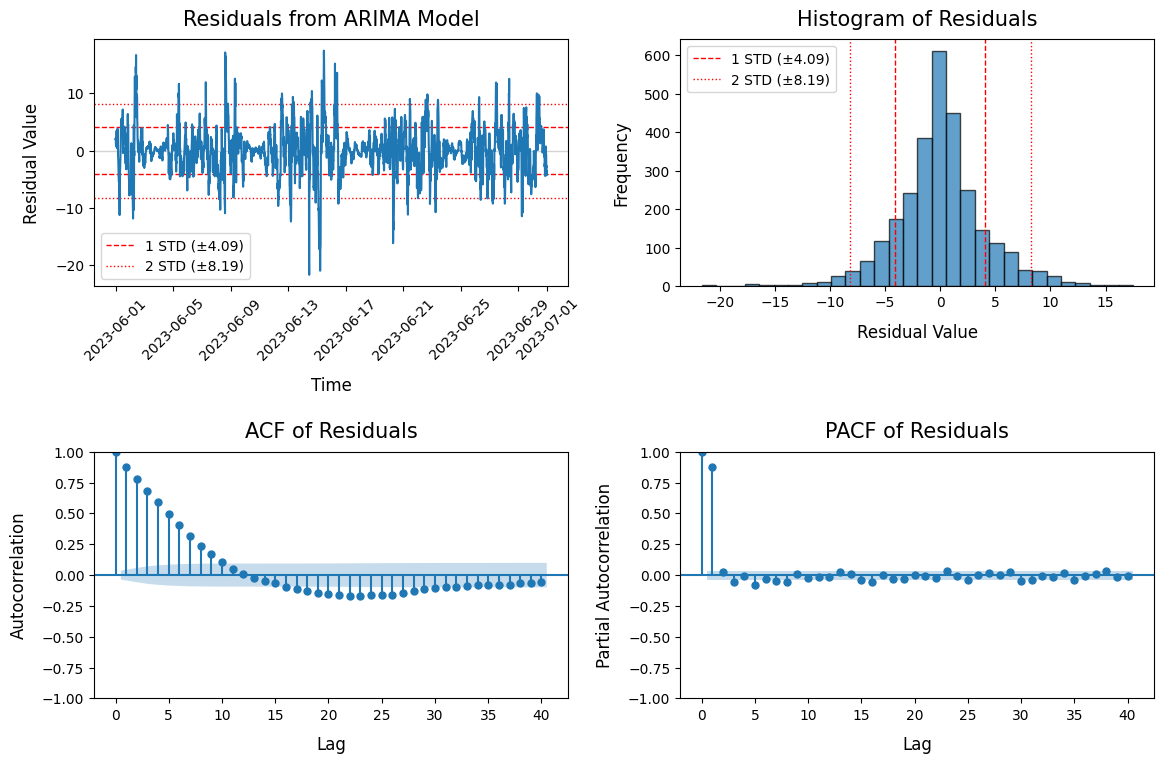
Evaluate Classification Model#
dw.eval_model() produces a detailed evaluation report for a classification model.
This function provides a comprehensive evaluation of a binary or multi-class classification model based on y_test (the actual target values) and y_pred (the predicted target values). It displays a text-based classification report enhanced with True/False Positives/Negatives, and 4 charts if plot is True: Confusion Matrix, Histogram of Predicted Probabilities, ROC Curve, and Precision-Recall Curve.
If class_type is ‘binary’ (default), it will treat this as a binary classification. If class_type is ‘multi’, it will treat this as a multi-class problem. To plot the curves or adjust the threshold (default 0.5), both X_test and estimator must be provided.
A number of classification metrics are shown in the report: Accuracy, Precision, Recall, F1, and ROC AUC. In addition, for binary classification, True Positive Rate, False Positive Rate, True Negative Rate, and False Negative Rate are shown.
Use this function to assess the performance of a trained classification model. You can experiment with different thresholds to see how they affect metrics like Precision, Recall, False Positive Rate and False Negative Rate. The plots make it easy to see if you’re getting good separation and maximum area under the curve.
Separate X and Y#
Let’s load the Bank dataset, which was already split into X and y. It’s a binary classification dataset. y is either ‘0’ or ‘1’.
[119]:
# Load the Bank dataset, already separated into X and y
X = pd.read_csv('data/X_bank.csv').drop(columns=['Unnamed: 0'])
y = pd.read_csv('data/y_bank.csv').drop(columns=['Unnamed: 0'])
[120]:
# Verify X/Y split
print(f'X: {X.shape}, y: {y.shape}')
X: (40195, 57), y: (40195, 1)
[121]:
# Verify X/Y columns
print(f'X: ({len(X.columns)})', list(X.columns))
print(f'y: ({len(y.columns)})', list(y.columns))
X: (57) ['age', 'duration', 'campaign', 'pdays', 'previous', 'emp.var.rate', 'cons.price.idx', 'cons.conf.idx', 'euribor3m', 'nr.employed', 'previously_contacted', 'job_admin.', 'job_blue-collar', 'job_entrepreneur', 'job_housemaid', 'job_management', 'job_retired', 'job_self-employed', 'job_services', 'job_student', 'job_technician', 'job_unemployed', 'job_unknown', 'marital_divorced', 'marital_married', 'marital_single', 'marital_unknown', 'education_basic.4y', 'education_basic.6y', 'education_basic.9y', 'education_high.school', 'education_illiterate', 'education_professional.course', 'education_university.degree', 'education_unknown', 'month_apr', 'month_aug', 'month_dec', 'month_jul', 'month_jun', 'month_mar', 'month_may', 'month_nov', 'month_oct', 'month_sep', 'day_of_week_fri', 'day_of_week_mon', 'day_of_week_thu', 'day_of_week_tue', 'day_of_week_wed', 'poutcome_failure', 'poutcome_nonexistent', 'poutcome_success', 'no_default_1', 'housing_yes', 'loan_yes', 'contact_telephone']
y: (1) ['subscribed_enc']
[122]:
# Set column lists
x_columns = list(X.columns)
y_columns = list(y.columns)
num_columns = x_columns
cat_columns = []
Split Train and Test#
Now we’ll separate the train set from the test set.
[123]:
# Create training and test datasets
X_train, X_test, y_train, y_test = train_test_split(X, y, test_size=0.25, random_state=42)
[124]:
# Verify train/test split
print('X:', X_train.shape, X_test.shape, y_train.shape, y_test.shape)
X: (30146, 57) (10049, 57) (30146, 1) (10049, 1)
Build a Pipeline#
[125]:
# Create a pipeline with Standard Scaler and Logistic Regression
pipe = dw.create_pipeline(scaler_key='stand', model_key='logreg', class_weight='balanced',
num_columns=num_columns, cat_columns=cat_columns)
[126]:
# Review the pipeline
pipe
[126]:
Pipeline(steps=[('stand', StandardScaler()),
('logreg',
LogisticRegression(class_weight='balanced', max_iter=10000,
random_state=42))])In a Jupyter environment, please rerun this cell to show the HTML representation or trust the notebook. On GitHub, the HTML representation is unable to render, please try loading this page with nbviewer.org.
Pipeline(steps=[('stand', StandardScaler()),
('logreg',
LogisticRegression(class_weight='balanced', max_iter=10000,
random_state=42))])StandardScaler()
LogisticRegression(class_weight='balanced', max_iter=10000, random_state=42)
Fit the Data#
[127]:
# Fit the pipeline with the training data, after adjusting y_train shape
pipe.fit(X_train, np.ravel(y_train))
[127]:
Pipeline(steps=[('stand', StandardScaler()),
('logreg',
LogisticRegression(class_weight='balanced', max_iter=10000,
random_state=42))])In a Jupyter environment, please rerun this cell to show the HTML representation or trust the notebook. On GitHub, the HTML representation is unable to render, please try loading this page with nbviewer.org.
Pipeline(steps=[('stand', StandardScaler()),
('logreg',
LogisticRegression(class_weight='balanced', max_iter=10000,
random_state=42))])StandardScaler()
LogisticRegression(class_weight='balanced', max_iter=10000, random_state=42)
Make Predictions#
[128]:
# Make predictions with the test data
y_pred = pipe.predict(X_test)
Evaluate Model Performance#
Let’s now use dw.eval_model to evaluate a classification model’s performance. Let’s start with a basic summary that doesn’t require the model and X_test to be passed, and then move on to examples that show charts and have customized values.
[129]:
# Create a dictionary of class labels to display names
class_map = {0: 'Declined', 1: 'Subscribed'}
[130]:
# Evaluate classification predictions with basic defaults
dw.eval_model(y_test=y_test, y_pred=y_pred, model_name='LogReg', pos_label=1, class_map=class_map)
LogReg Binary Classification Report
precision recall f1-score support
Declined 0.98 0.86 0.92 8872
Subscribed 0.46 0.89 0.61 1177
accuracy 0.86 10049
macro avg 0.72 0.88 0.76 10049
weighted avg 0.92 0.86 0.88 10049
Predicted:0 1
Actual: 0 7636 1236
Actual: 1 128 1049
True Positive Rate / Sensitivity: 0.89
True Negative Rate / Specificity: 0.86
False Positive Rate / Fall-out: 0.14
False Negative Rate / Miss Rate: 0.11
Positive Class: Subscribed (1)
Threshold: 0.5
[131]:
# Evaluate classification model with charting enabled, and passing X_test and estimator for proababilities
dw.eval_model(y_test=y_test, y_pred=y_pred, x_test=X_test, estimator=pipe, model_name='LogReg',
pos_label=1, class_map=class_map, plot=True)
LogReg Binary Classification Report
precision recall f1-score support
Declined 0.98 0.86 0.92 8872
Subscribed 0.46 0.89 0.61 1177
accuracy 0.86 10049
macro avg 0.72 0.88 0.76 10049
weighted avg 0.92 0.86 0.88 10049
ROC AUC: 0.94
Predicted:0 1
Actual: 0 7636 1236
Actual: 1 128 1049
True Positive Rate / Sensitivity: 0.89
True Negative Rate / Specificity: 0.86
False Positive Rate / Fall-out: 0.14
False Negative Rate / Miss Rate: 0.11
Positive Class: Subscribed (1)
Threshold: 0.5
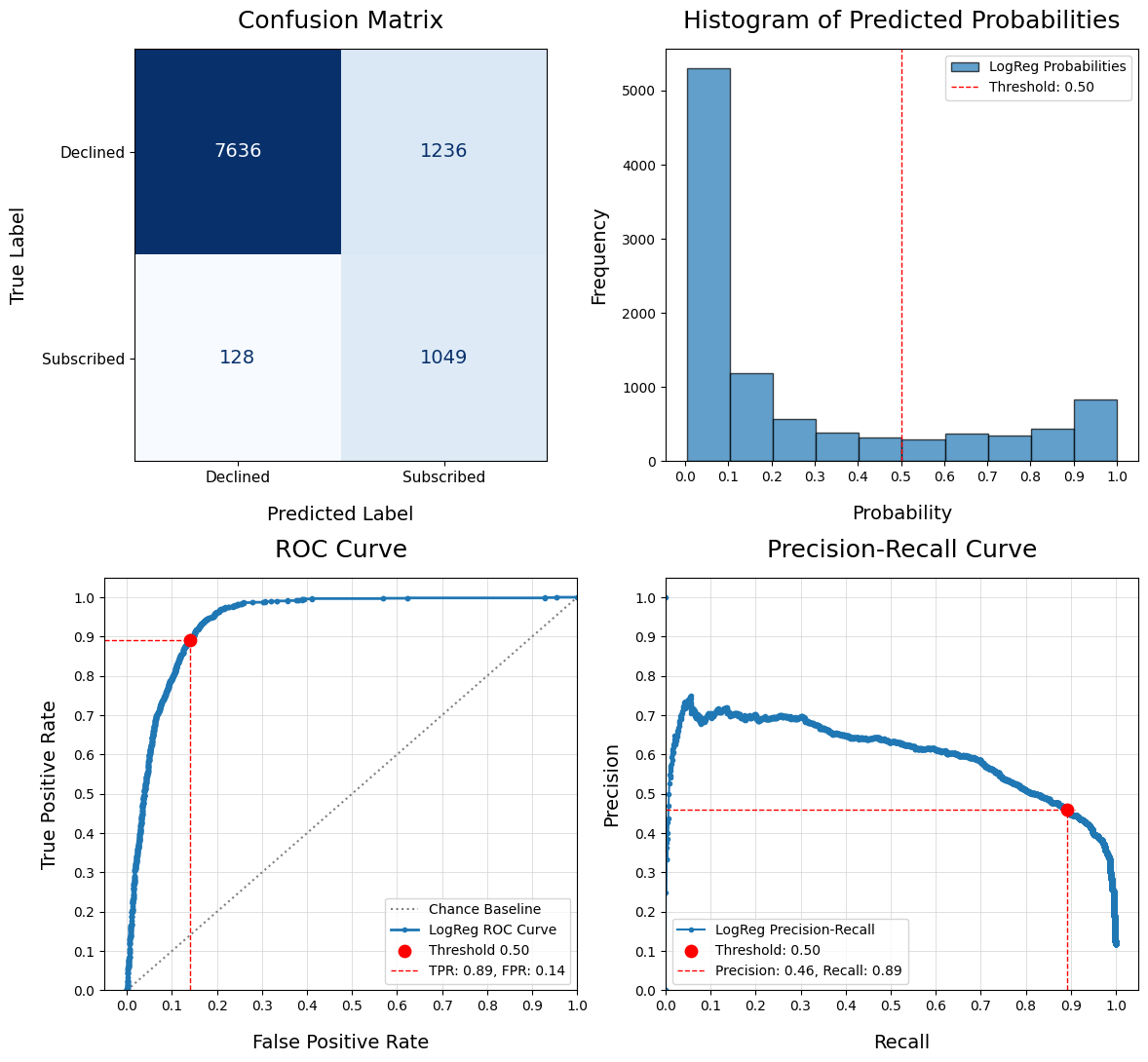
[132]:
# Evaluate classification model with charting, custom threshold, and return metrics
class_metrics = dw.eval_model(y_test=y_test, y_pred=y_pred, x_test=X_test, estimator=pipe, model_name='LogReg',
pos_label=1, class_map=class_map, plot=True, bins=20, threshold=0.35, return_metrics=True)
LogReg Binary Classification Report
precision recall f1-score support
Declined 0.99 0.81 0.89 8872
Subscribed 0.40 0.95 0.56 1177
accuracy 0.83 10049
macro avg 0.70 0.88 0.73 10049
weighted avg 0.92 0.83 0.85 10049
ROC AUC: 0.94
Predicted:0 1
Actual: 0 7189 1683
Actual: 1 58 1119
True Positive Rate / Sensitivity: 0.95
True Negative Rate / Specificity: 0.81
False Positive Rate / Fall-out: 0.19
False Negative Rate / Miss Rate: 0.05
Positive Class: Subscribed (1)
Threshold: 0.35

[133]:
# Review the extracted metrics
class_metrics
[133]:
{'True Positives': 1119,
'False Positives': 1683,
'True Negatives': 7189,
'False Negatives': 58,
'TPR': 0.9507221750212405,
'TNR': 0.8103020739404869,
'FPR': 0.18969792605951308,
'FNR': 0.04927782497875956,
'Declined': {'precision': 0.9919966882848075,
'recall': 0.8103020739404869,
'f1-score': 0.8919908182889758,
'support': 8872.0},
'Subscribed': {'precision': 0.3993576017130621,
'recall': 0.9507221750212405,
'f1-score': 0.562452877607439,
'support': 1177.0},
'accuracy': 0.8267489302418151,
'macro avg': {'precision': 0.6956771449989347,
'recall': 0.8805121244808637,
'f1-score': 0.7272218479482073,
'support': 10049.0},
'weighted avg': {'precision': 0.9225831939177117,
'recall': 0.8267489302418151,
'f1-score': 0.8533933303616029,
'support': 10049.0},
'ROC AUC': 0.9387968831519055,
'Threshold': 0.35,
'Class Type': 'binary',
'Class Map': {0: 'Declined', 1: 'Subscribed'},
'Positive Label': 1,
'Title': None,
'Model Name': 'LogReg',
'Class Weight': None,
'Multi-Class': 'ovr',
'Average': 'macro'}
Multi-Class Example#
Let’s take a look at a mult-class classification dataset, where there are more than 2 classes. In this case, we won’t see all the charts you get with binary classification. But we will see the classification report, and confusion matrix. And we’ll see an ROC AUC score if the X_test and estimator are provided.
[134]:
# Load Iris dataset for multi-class example
X2, y2 = load_iris(return_X_y=True)
X2 = pd.DataFrame(X2, columns=['sepal_length', 'sepal_width', 'petal_length', 'petal_width'])
y2 = pd.Series(y2)
X2_train, X2_test, y2_train, y2_test = train_test_split(X2, y2, test_size=0.2, random_state=42)
class_map2 = {0: 'Setosa', 1: 'Versicolor', 2: 'Virginica'}
model2 = SVC(kernel='linear', probability=True, random_state=42)
model2.fit(X2_train, y2_train)
SVC(kernel='linear', probability=True, random_state=42)
y2_pred = model2.predict(X2_test)
[135]:
# Evaluate a multi-class model, plot the charts, and return the metrics
multi_metrics = dw.eval_model(y_test=y2_test, y_pred=y2_pred, x_test=X2_test, estimator=model2,
class_map=class_map2, return_metrics=True, plot=True)
Multi-Class Classification Report
precision recall f1-score support
Setosa 1.00 1.00 1.00 10
Versicolor 1.00 1.00 1.00 9
Virginica 1.00 1.00 1.00 11
accuracy 1.00 30
macro avg 1.00 1.00 1.00 30
weighted avg 1.00 1.00 1.00 30
ROC AUC: 1.0
Predicted Setosa Versicolor Virginica
Actual
Setosa 10 0 0
Versicolor 0 9 0
Virginica 0 0 11
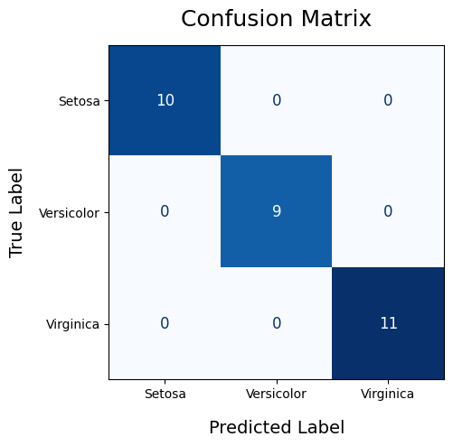
[136]:
# Review the extracted metrics
multi_metrics
[136]:
{'Setosa': {'precision': 1.0, 'recall': 1.0, 'f1-score': 1.0, 'support': 10.0},
'Versicolor': {'precision': 1.0,
'recall': 1.0,
'f1-score': 1.0,
'support': 9.0},
'Virginica': {'precision': 1.0,
'recall': 1.0,
'f1-score': 1.0,
'support': 11.0},
'accuracy': 1.0,
'macro avg': {'precision': 1.0,
'recall': 1.0,
'f1-score': 1.0,
'support': 30.0},
'weighted avg': {'precision': 1.0,
'recall': 1.0,
'f1-score': 1.0,
'support': 30.0},
'ROC AUC': 1.0,
'Threshold': 0.5,
'Class Type': 'multi',
'Class Map': {0: 'Setosa', 1: 'Versicolor', 2: 'Virginica'},
'Positive Label': None,
'Title': None,
'Model Name': 'Model',
'Class Weight': None,
'Multi-Class': 'ovr',
'Average': 'macro'}
Compare Models#
dw.compare models() finds the best classification model and hyper-parameters for a dataset by automating the workflow for multiple models and comparing results.
This function integrates a number of steps in a typical classification model workflow, and it does this for multiple models, all with one command line:
Auto-detecting single vs. multi-class classification problems
Option to Under-sample or Over-smple imbalanced data,
Option to use a sub-sample of data for SVC or KNN, which can be computation intense
Ability to split the Train/Test data at a specified ratio,
Creation of a multiple-step Pipeline, including Imputation, multiple Column Transformer/Encoding steps, Scaling, Feature selection, and the Model,
Grid Search of hyper-parameters, either full or random,
Calculating performance metrics from the standard Classification Report (Accuracy, Precision, Recall, F1) but also with ROC AUC, and if binary, True Positive Rate, True Negative Rate, False Positive Rate, False Negative Rate,
Evaluating this performance based on a customizable Threshold,
Visually showing performance by plotting (a) a Confusion Matrix, and if binary, (b) a Histogram of Predicted Probabilities, (c) an ROC Curve, and (d) a Precision-Recall Curve.
Save all the results in a DataFrame for reference and comparison, and
Option to plot the results to visually compare performance of the specified metric across multiple model pipelines with their best parameters.
To use this function, a configuration should be created that defines the desired model configurations and parameters you want to search. When compare_models is run, for each model in the models parameter, the create_pipeline function will be called to create a pipeline from the specified parameters. Each model iteration will have the same pipeline construction, except for the final model, which will vary. Here are the major pipeline parameters, along with the config sections they map
to:
imputer(str) is selected fromconfig['imputers']transformers(list or str) are selected fromconfig['transformers']scaler(str) is selected fromconfig['scalers']selector(str) is selected fromconfig['selectors']models(list or str) are selected fromconfig['models']
Here is an example of the configuration dictionary structure. It is based on what create_pipeline requires to assemble the pipeline. But it adds some additional configuration parameters referenced by compare_models, which are params (grid search parameters, required) and cv (cross-validation parameters, optional if grid_cv is an integer). The configuration dictionary is passed to compare_models as the config parameter:
>>> config = { # doctest: +SKIP
... 'imputers': {
... 'knn_imputer': KNNImputer().set_output(transform='pandas'),
... 'simple_imputer': SimpleImputer()
... },
... 'transformers': {
... 'ohe': (OneHotEncoder(drop='if_binary', handle_unknown='ignore'),
... cat_columns),
... 'ord': (OrdinalEncoder(), cat_columns),
... 'poly2': (PolynomialFeatures(degree=2, include_bias=False),
... num_columns),
... 'log': (FunctionTransformer(np.log1p, validate=True),
... num_columns)
... },
... 'scalers': {
... 'stand': StandardScaler(),
... 'minmax': MinMaxScaler()
... },
... 'selectors': {
... 'rfe_logreg': RFE(LogisticRegression(max_iter=max_iter,
... random_state=random_state,
... class_weight=class_weight)),
... 'sfs_linreg': SequentialFeatureSelector(LinearRegression())
... },
... 'models': {
... 'linreg': LinearRegression(),
... 'logreg': LogisticRegression(max_iter=max_iter,
... random_state=random_state,
... class_weight=class_weight),
... 'tree_class': DecisionTreeClassifier(random_state=random_state),
... 'tree_reg': DecisionTreeRegressor(random_state=random_state)
... },
... 'no_scale': ['tree_class', 'tree_reg'],
... 'no_poly': ['tree_class', 'tree_reg'],
... 'params': {
... 'sfs': {
... 'Selector: sfs__n_features_to_select': np.arange(3, 13, 1),
... },
... 'linreg': {
... 'Model: linreg__fit_intercept': [True],
... },
... 'ridge': {
... 'Model: ridge__alpha': np.array([0.01, 0.1, 1, 10, 100, 1000]),
... }
... },
... 'cv': {
... 'kfold_5': KFold(n_splits=5, shuffle=True, random_state=42),
... 'skf_5': StratifiedKFold(n_splits=5, shuffle=True, random_state=42),
... }
... }
In addition to the configuration file, you will need to define any column lists if you want to target certain transformations to a subset of columns. For example, you might define a ‘ohe’ transformer for One-Hot Encoding, and reference ‘ohe_columns’ or ‘cat_columns’ in its definition in the config.
Here is an example of how to call this function in an organized manner:
>>> results_df = dw.compare_models( # doctest: +SKIP
...
... # Data split and sampling
... x=X, y=y, test_size=0.25, stratify=None, under_sample=None,
... over_sample=None, svm_knn_resample=None,
...
... # Models and pipeline steps
... imputer=None, transformers=None, scaler='stand', selector=None,
... models=['logreg', 'knn_class', 'svm_proba', 'tree_class',
... 'forest_class', 'xgb_class', 'keras_class'], svm_proba=True,
...
... # Grid search
... search_type='random', scorer='accuracy', grid_cv='kfold_5', verbose=4,
...
... # Model evaluation and charts
... model_eval=True, plot_perf=True, plot_curve=True, fig_size=(12,6),
... legend_loc='lower left', rotation=45, threshold=0.5,
... class_map=class_map, pos_label=1, title='Breast Cancer',
...
... # Config, preferences and notes
... config=my_config, class_weight=None, random_state=42, decimal=4,
... n_jobs=None, debug=False, notes='Test Size=0.25, Threshold=0.50'
... )
Use this function when you want to find the best classification model and hyper-parameters for a dataset, after doing any required pre-processing or cleaning. It is a significant time saver, replacing numerous manual coding steps with one command.
Load and Prepare Data#
Let’s load a simple binary classification dataset to illustrate how easy it is to compare multiple classification models using this function.
[137]:
# Load breast cancer data
cancer_df = pd.read_csv('data/breast_cancer.csv', index_col=0).drop(columns='Unnamed: 32')
[138]:
# Review the data
cancer_df[:5]
[138]:
| diagnosis | radius_mean | texture_mean | perimeter_mean | area_mean | smoothness_mean | compactness_mean | concavity_mean | concave points_mean | symmetry_mean | fractal_dimension_mean | radius_se | texture_se | perimeter_se | area_se | smoothness_se | compactness_se | concavity_se | concave points_se | symmetry_se | fractal_dimension_se | radius_worst | texture_worst | perimeter_worst | area_worst | smoothness_worst | compactness_worst | concavity_worst | concave points_worst | symmetry_worst | fractal_dimension_worst | |
|---|---|---|---|---|---|---|---|---|---|---|---|---|---|---|---|---|---|---|---|---|---|---|---|---|---|---|---|---|---|---|---|
| id | |||||||||||||||||||||||||||||||
| 842302 | M | 17.99 | 10.38 | 122.80 | 1001.0 | 0.11840 | 0.27760 | 0.3001 | 0.14710 | 0.2419 | 0.07871 | 1.0950 | 0.9053 | 8.589 | 153.40 | 0.006399 | 0.04904 | 0.05373 | 0.01587 | 0.03003 | 0.006193 | 25.38 | 17.33 | 184.60 | 2019.0 | 0.1622 | 0.6656 | 0.7119 | 0.2654 | 0.4601 | 0.11890 |
| 842517 | M | 20.57 | 17.77 | 132.90 | 1326.0 | 0.08474 | 0.07864 | 0.0869 | 0.07017 | 0.1812 | 0.05667 | 0.5435 | 0.7339 | 3.398 | 74.08 | 0.005225 | 0.01308 | 0.01860 | 0.01340 | 0.01389 | 0.003532 | 24.99 | 23.41 | 158.80 | 1956.0 | 0.1238 | 0.1866 | 0.2416 | 0.1860 | 0.2750 | 0.08902 |
| 84300903 | M | 19.69 | 21.25 | 130.00 | 1203.0 | 0.10960 | 0.15990 | 0.1974 | 0.12790 | 0.2069 | 0.05999 | 0.7456 | 0.7869 | 4.585 | 94.03 | 0.006150 | 0.04006 | 0.03832 | 0.02058 | 0.02250 | 0.004571 | 23.57 | 25.53 | 152.50 | 1709.0 | 0.1444 | 0.4245 | 0.4504 | 0.2430 | 0.3613 | 0.08758 |
| 84348301 | M | 11.42 | 20.38 | 77.58 | 386.1 | 0.14250 | 0.28390 | 0.2414 | 0.10520 | 0.2597 | 0.09744 | 0.4956 | 1.1560 | 3.445 | 27.23 | 0.009110 | 0.07458 | 0.05661 | 0.01867 | 0.05963 | 0.009208 | 14.91 | 26.50 | 98.87 | 567.7 | 0.2098 | 0.8663 | 0.6869 | 0.2575 | 0.6638 | 0.17300 |
| 84358402 | M | 20.29 | 14.34 | 135.10 | 1297.0 | 0.10030 | 0.13280 | 0.1980 | 0.10430 | 0.1809 | 0.05883 | 0.7572 | 0.7813 | 5.438 | 94.44 | 0.011490 | 0.02461 | 0.05688 | 0.01885 | 0.01756 | 0.005115 | 22.54 | 16.67 | 152.20 | 1575.0 | 0.1374 | 0.2050 | 0.4000 | 0.1625 | 0.2364 | 0.07678 |
[139]:
# Separate X and y
X = cancer_df.drop(columns='diagnosis')
y = cancer_df['diagnosis']
Identify Class Labels#
To make sure we know the display names for the values or labels in ‘y’, a class_map dictionary shoudl be created. For binary classification, we will need to specify which of these labels represents the positive class as the pos_label parameter.
[140]:
# Encode to numeric values for XGB classifier
mapping_dict = {'M': 1, 'B': 0}
y_enc = y.map(mapping_dict)
# Map class labels to display names
class_map = {0: 'Benign', 1: 'Malignant'}
Define Configuration#
A configuration dictionary needs to be created, and it will require all the reference libraries to be imported, and any column lists or variable names to be defined.
[141]:
# Set some variables referenced in the config
random_state = 42
class_weight = None
max_iter = 10000
# Set column lists referenced in the config
num_columns = list(X.columns)
cat_columns = []
ohe_columns = []
ord_columns = []
poly2_columns = []
log_columns = []
# If you are doing One-Hot Encoding, you might specify a value to drop
ohe_drop_value = []
# If you are doing ordinal encoding, the ordering needs to be specified
ord_category_order = [[]]
# Define the callback for early stop, referenced by KerasClassifier
stopper = EarlyStopping(patience=4)
# Create a custom configuration file with model pipeline components and grid search params
my_config = {
'models' : {
'logreg': LogisticRegression(max_iter=max_iter, random_state=random_state, class_weight=class_weight),
'knn_class': KNeighborsClassifier(),
'svm': SVC(random_state=random_state, probability=False, class_weight=class_weight),
'svm_proba': SVC(random_state=random_state, probability=True, class_weight=class_weight),
'tree_class': DecisionTreeClassifier(random_state=random_state, class_weight=class_weight),
'forest_class': RandomForestClassifier(random_state=random_state, class_weight=class_weight),
'xgb_class': XGBClassifier(random_state=random_state),
'keras_class': KerasClassifier(model=dw.create_nn_binary, hidden_layer_dim=50, second_layer_dim=None,
third_layer_dim=None, dropout_rate=0.2, epochs=50, l2_reg=0.0,
verbose=0, class_weight=class_weight, random_state=random_state,
fit__validation_split=0.2, fit__callbacks=[stopper],
fit__batch_size=32, metrics=['accuracy'])
},
'imputers': {
'knn_imputer': KNNImputer().set_output(transform='pandas'),
'simple_imputer': SimpleImputer()
},
'transformers': {
'ohe': (OneHotEncoder(drop='if_binary', handle_unknown='ignore'), ohe_columns),
'ohe_drop': (OneHotEncoder(drop=ohe_drop_value, handle_unknown='ignore'), ohe_columns),
'ord': (OrdinalEncoder(categories=ord_category_order), ord_columns),
'poly2': (PolynomialFeatures(degree=2, include_bias=False), poly2_columns),
'log': (LogTransformer(), log_columns),
},
'scalers': {
'stand': StandardScaler(),
'robust': RobustScaler(),
'minmax': MinMaxScaler()
},
'selectors': {
'rfe_logreg': RFE(LogisticRegression(max_iter=max_iter, random_state=random_state,
class_weight=class_weight)),
'sfs_logreg': SequentialFeatureSelector(LogisticRegression(max_iter=max_iter, random_state=random_state,
class_weight=class_weight))
},
'params' : {
'logreg': {
'logreg__C': [0.0001, 0.001, 0.01, 0.1, 1, 10, 100],
'logreg__solver': ['newton-cg', 'lbfgs', 'saga']
},
'knn_class': {
'knn_class__n_neighbors': [3, 5, 10, 15, 20, 25],
'knn_class__weights': ['uniform', 'distance'],
'knn_class__metric': ['euclidean', 'manhattan']
},
'svm': {
'svm__C': [0.0001, 0.001, 0.01, 0.1, 1, 10, 100],
'svm__kernel': ['linear', 'poly', 'rbf', 'sigmoid']
},
'svm_proba': {
'svm_proba__C': [0.0001, 0.001, 0.01, 0.1, 1, 10, 100],
'svm_proba__kernel': ['linear', 'poly', 'rbf', 'sigmoid']
},
'tree_class': {
'tree_class__max_depth': [3, 5, 7],
'tree_class__min_samples_split': [5, 10, 15],
'tree_class__criterion': ['gini', 'entropy'],
'tree_class__min_samples_leaf': [2, 4, 6]
},
'forest_class': {
'forest_class__n_estimators' : [50, 100, 200],
'forest_class__max_depth': [3, 5, 7],
'forest_class__min_samples_split': [5, 10, 15],
'forest_class__criterion': ['gini', 'entropy'],
'forest_class__min_samples_leaf': [2, 4, 6]
},
'xgb_class': {
'xgb_class__learning_rate': [0.01, 0.1, 0.5],
'xgb_class__max_depth': [3, 5, 7],
'xgb_class__subsample': [0.7, 0.8, 0.9],
'xgb_class__colsample_bytree': [0.7, 0.8, 0.9],
'xgb_class__n_estimators': [50, 100, 200],
'xgb_class__objective': ['binary:logistic'],
'xgb_class__gamma': [0, 1, 5, 10]
},
'keras_class': {
'keras_class__loss': ['binary_crossentropy'],
'keras_class__optimizer': ['adam'],
'keras_class__hidden_layer_dim': [50, 100, 200],
'keras_class__dropout_rate': [0.5],
'keras_class__l2_reg': [0.0],
'keras_class__second_layer_dim': [50, 100],
'keras_class__third_layer_dim': [None, 25, 50],
'keras_class__optimizer__learning_rate': [0.001],
'keras_class__fit__batch_size': [32]
},
},
'cv': {
'kfold_3': KFold(n_splits=3, shuffle=True, random_state=42),
'kfold_5': KFold(n_splits=5, shuffle=True, random_state=42),
'skf_5': StratifiedKFold(n_splits=5, shuffle=True, random_state=42),
},
'no_scale': ['tree_class', 'forest_class'],
'no_poly': ['knn_class', 'tree_class', 'forest_class', 'xgb_class']
}
Compare Binary Classification Models#
Let’s now automatically build the same pipeline for 7 different models, perform a grid search to find the best hyper-parameters, capture a number of binary classification metrics, and plot the model’s performance visually. Everything will be stored in the ‘results_df’ DataFrame so we can further anaylize or plot the metrics.
[142]:
# Evaluate multiple classification models by searching for the best hyper-parameters and comparing results
results_df = dw.compare_models(
# Data split and sampling
x=X, y=y_enc, test_size=0.25, stratify=None, under_sample=None, over_sample=None, svm_knn_resample=None,
# Models and pipeline steps
imputer=None, transformers=None, scaler='stand', selector=None, svm_proba=True,
models=['logreg', 'knn_class', 'svm_proba', 'tree_class', 'forest_class', 'xgb_class', 'keras_class'],
# Grid search
search_type='random', scorer='accuracy', grid_cv='kfold_5', verbose=4,
# Model evaluation and charts
model_eval=True, plot_perf=True, plot_curve=True, fig_size=(12,6), legend_loc='lower left', rotation=45,
threshold=0.5, class_map=class_map, pos_label=1, title='Breast Cancer',
# Config, preferences and notes
config=my_config, class_weight=None, random_state=42, decimal=4, n_jobs=None,
notes='X, Test Size=0.25, Standard Scaler, Random Grid (Accuracy), T=0.50'
)
-----------------------------------------------------------------------------------------
Starting Data Processing - May 30, 2024 09:18 AM UTC
-----------------------------------------------------------------------------------------
Classification type detected: binary
Unique values in y: [0 1]
Train/Test split, test_size: 0.25
X_train, X_test, y_train, y_test shapes: (426, 30) (143, 30) (426,) (143,)
-----------------------------------------------------------------------------------------
1/7: Starting LogisticRegression Random Search - May 30, 2024 09:18 AM UTC
-----------------------------------------------------------------------------------------
Fitting 5 folds for each of 10 candidates, totalling 50 fits
[CV 1/5] END logreg__C=0.0001, logreg__solver=newton-cg;, score=0.733 total time= 0.0s
[CV 2/5] END logreg__C=0.0001, logreg__solver=newton-cg;, score=0.612 total time= 0.0s
[CV 3/5] END logreg__C=0.0001, logreg__solver=newton-cg;, score=0.682 total time= 0.0s
[CV 4/5] END logreg__C=0.0001, logreg__solver=newton-cg;, score=0.588 total time= 0.0s
[CV 5/5] END logreg__C=0.0001, logreg__solver=newton-cg;, score=0.565 total time= 0.0s
[CV 1/5] END .logreg__C=10, logreg__solver=saga;, score=1.000 total time= 0.3s
[CV 2/5] END .logreg__C=10, logreg__solver=saga;, score=0.929 total time= 0.3s
[CV 3/5] END .logreg__C=10, logreg__solver=saga;, score=0.988 total time= 0.3s
[CV 4/5] END .logreg__C=10, logreg__solver=saga;, score=0.988 total time= 0.2s
[CV 5/5] END .logreg__C=10, logreg__solver=saga;, score=0.976 total time= 0.3s
[CV 1/5] END logreg__C=10, logreg__solver=newton-cg;, score=1.000 total time= 0.0s
[CV 2/5] END logreg__C=10, logreg__solver=newton-cg;, score=0.929 total time= 0.0s
[CV 3/5] END logreg__C=10, logreg__solver=newton-cg;, score=0.988 total time= 0.0s
[CV 4/5] END logreg__C=10, logreg__solver=newton-cg;, score=0.988 total time= 0.0s
[CV 5/5] END logreg__C=10, logreg__solver=newton-cg;, score=0.976 total time= 0.0s
[CV 1/5] END logreg__C=0.0001, logreg__solver=lbfgs;, score=0.733 total time= 0.0s
[CV 2/5] END logreg__C=0.0001, logreg__solver=lbfgs;, score=0.612 total time= 0.0s
[CV 3/5] END logreg__C=0.0001, logreg__solver=lbfgs;, score=0.682 total time= 0.0s
[CV 4/5] END logreg__C=0.0001, logreg__solver=lbfgs;, score=0.588 total time= 0.0s
[CV 5/5] END logreg__C=0.0001, logreg__solver=lbfgs;, score=0.565 total time= 0.0s
[CV 1/5] END logreg__C=0.01, logreg__solver=saga;, score=0.965 total time= 0.0s
[CV 2/5] END logreg__C=0.01, logreg__solver=saga;, score=0.871 total time= 0.0s
[CV 3/5] END logreg__C=0.01, logreg__solver=saga;, score=1.000 total time= 0.0s
[CV 4/5] END logreg__C=0.01, logreg__solver=saga;, score=0.953 total time= 0.0s
[CV 5/5] END logreg__C=0.01, logreg__solver=saga;, score=0.929 total time= 0.0s
[CV 1/5] END logreg__C=0.001, logreg__solver=saga;, score=0.930 total time= 0.0s
[CV 2/5] END logreg__C=0.001, logreg__solver=saga;, score=0.812 total time= 0.0s
[CV 3/5] END logreg__C=0.001, logreg__solver=saga;, score=0.965 total time= 0.0s
[CV 4/5] END logreg__C=0.001, logreg__solver=saga;, score=0.859 total time= 0.0s
[CV 5/5] END logreg__C=0.001, logreg__solver=saga;, score=0.871 total time= 0.0s
[CV 1/5] END logreg__C=0.1, logreg__solver=saga;, score=0.988 total time= 0.0s
[CV 2/5] END logreg__C=0.1, logreg__solver=saga;, score=0.906 total time= 0.0s
[CV 3/5] END logreg__C=0.1, logreg__solver=saga;, score=1.000 total time= 0.0s
[CV 4/5] END logreg__C=0.1, logreg__solver=saga;, score=0.988 total time= 0.0s
[CV 5/5] END logreg__C=0.1, logreg__solver=saga;, score=0.965 total time= 0.0s
[CV 1/5] END logreg__C=0.001, logreg__solver=newton-cg;, score=0.930 total time= 0.0s
[CV 2/5] END logreg__C=0.001, logreg__solver=newton-cg;, score=0.812 total time= 0.0s
[CV 3/5] END logreg__C=0.001, logreg__solver=newton-cg;, score=0.965 total time= 0.0s
[CV 4/5] END logreg__C=0.001, logreg__solver=newton-cg;, score=0.859 total time= 0.0s
[CV 5/5] END logreg__C=0.001, logreg__solver=newton-cg;, score=0.871 total time= 0.0s
[CV 1/5] END logreg__C=100, logreg__solver=newton-cg;, score=0.977 total time= 0.0s
[CV 2/5] END logreg__C=100, logreg__solver=newton-cg;, score=0.929 total time= 0.0s
[CV 3/5] END logreg__C=100, logreg__solver=newton-cg;, score=0.988 total time= 0.0s
[CV 4/5] END logreg__C=100, logreg__solver=newton-cg;, score=0.965 total time= 0.0s
[CV 5/5] END logreg__C=100, logreg__solver=newton-cg;, score=0.988 total time= 0.0s
[CV 1/5] END logreg__C=10, logreg__solver=lbfgs;, score=1.000 total time= 0.0s
[CV 2/5] END logreg__C=10, logreg__solver=lbfgs;, score=0.929 total time= 0.0s
[CV 3/5] END logreg__C=10, logreg__solver=lbfgs;, score=0.988 total time= 0.0s
[CV 4/5] END logreg__C=10, logreg__solver=lbfgs;, score=0.988 total time= 0.0s
[CV 5/5] END logreg__C=10, logreg__solver=lbfgs;, score=0.976 total time= 0.0s
Total Time: 2.6005 seconds
Average Fit Time: 0.0520 seconds
Inference Time: 0.0013
Best CV Accuracy Score: 0.9765
Train Accuracy Score: 0.9906
Test Accuracy Score: 0.9720
Overfit: Yes
Overfit Difference: 0.0186
Best Parameters: {'logreg__solver': 'saga', 'logreg__C': 10}
LogisticRegression Binary Classification Report
precision recall f1-score support
Benign 0.9885 0.9663 0.9773 89
Malignant 0.9464 0.9815 0.9636 54
accuracy 0.9720 143
macro avg 0.9675 0.9739 0.9705 143
weighted avg 0.9726 0.9720 0.9721 143
ROC AUC: 0.9956
Predicted:0 1
Actual: 0 86 3
Actual: 1 1 53
True Positive Rate / Sensitivity: 0.9815
True Negative Rate / Specificity: 0.9663
False Positive Rate / Fall-out: 0.0337
False Negative Rate / Miss Rate: 0.0185
Positive Class: Malignant (1)
Threshold: 0.5

-----------------------------------------------------------------------------------------
2/7: Starting KNeighborsClassifier Random Search - May 30, 2024 09:18 AM UTC
-----------------------------------------------------------------------------------------
Fitting 5 folds for each of 10 candidates, totalling 50 fits
[CV 1/5] END knn_class__metric=euclidean, knn_class__n_neighbors=20, knn_class__weights=uniform;, score=0.965 total time= 0.1s
[CV 2/5] END knn_class__metric=euclidean, knn_class__n_neighbors=20, knn_class__weights=uniform;, score=0.859 total time= 0.0s
[CV 3/5] END knn_class__metric=euclidean, knn_class__n_neighbors=20, knn_class__weights=uniform;, score=0.988 total time= 0.0s
[CV 4/5] END knn_class__metric=euclidean, knn_class__n_neighbors=20, knn_class__weights=uniform;, score=0.965 total time= 0.0s
[CV 5/5] END knn_class__metric=euclidean, knn_class__n_neighbors=20, knn_class__weights=uniform;, score=0.941 total time= 0.0s
[CV 1/5] END knn_class__metric=manhattan, knn_class__n_neighbors=10, knn_class__weights=uniform;, score=0.965 total time= 0.0s
[CV 2/5] END knn_class__metric=manhattan, knn_class__n_neighbors=10, knn_class__weights=uniform;, score=0.882 total time= 0.0s
[CV 3/5] END knn_class__metric=manhattan, knn_class__n_neighbors=10, knn_class__weights=uniform;, score=1.000 total time= 0.0s
[CV 4/5] END knn_class__metric=manhattan, knn_class__n_neighbors=10, knn_class__weights=uniform;, score=0.976 total time= 0.0s
[CV 5/5] END knn_class__metric=manhattan, knn_class__n_neighbors=10, knn_class__weights=uniform;, score=0.953 total time= 0.0s
[CV 1/5] END knn_class__metric=euclidean, knn_class__n_neighbors=3, knn_class__weights=uniform;, score=0.988 total time= 0.0s
[CV 2/5] END knn_class__metric=euclidean, knn_class__n_neighbors=3, knn_class__weights=uniform;, score=0.882 total time= 0.0s
[CV 3/5] END knn_class__metric=euclidean, knn_class__n_neighbors=3, knn_class__weights=uniform;, score=1.000 total time= 0.0s
[CV 4/5] END knn_class__metric=euclidean, knn_class__n_neighbors=3, knn_class__weights=uniform;, score=0.988 total time= 0.0s
[CV 5/5] END knn_class__metric=euclidean, knn_class__n_neighbors=3, knn_class__weights=uniform;, score=0.976 total time= 0.0s
[CV 1/5] END knn_class__metric=manhattan, knn_class__n_neighbors=15, knn_class__weights=uniform;, score=0.977 total time= 0.0s
[CV 2/5] END knn_class__metric=manhattan, knn_class__n_neighbors=15, knn_class__weights=uniform;, score=0.894 total time= 0.0s
[CV 3/5] END knn_class__metric=manhattan, knn_class__n_neighbors=15, knn_class__weights=uniform;, score=1.000 total time= 0.0s
[CV 4/5] END knn_class__metric=manhattan, knn_class__n_neighbors=15, knn_class__weights=uniform;, score=0.965 total time= 0.0s
[CV 5/5] END knn_class__metric=manhattan, knn_class__n_neighbors=15, knn_class__weights=uniform;, score=0.929 total time= 0.0s
[CV 1/5] END knn_class__metric=euclidean, knn_class__n_neighbors=25, knn_class__weights=distance;, score=0.977 total time= 0.0s
[CV 2/5] END knn_class__metric=euclidean, knn_class__n_neighbors=25, knn_class__weights=distance;, score=0.882 total time= 0.0s
[CV 3/5] END knn_class__metric=euclidean, knn_class__n_neighbors=25, knn_class__weights=distance;, score=1.000 total time= 0.0s
[CV 4/5] END knn_class__metric=euclidean, knn_class__n_neighbors=25, knn_class__weights=distance;, score=0.965 total time= 0.0s
[CV 5/5] END knn_class__metric=euclidean, knn_class__n_neighbors=25, knn_class__weights=distance;, score=0.941 total time= 0.0s
[CV 1/5] END knn_class__metric=euclidean, knn_class__n_neighbors=20, knn_class__weights=distance;, score=0.977 total time= 0.0s
[CV 2/5] END knn_class__metric=euclidean, knn_class__n_neighbors=20, knn_class__weights=distance;, score=0.882 total time= 0.0s
[CV 3/5] END knn_class__metric=euclidean, knn_class__n_neighbors=20, knn_class__weights=distance;, score=0.988 total time= 0.0s
[CV 4/5] END knn_class__metric=euclidean, knn_class__n_neighbors=20, knn_class__weights=distance;, score=0.965 total time= 0.0s
[CV 5/5] END knn_class__metric=euclidean, knn_class__n_neighbors=20, knn_class__weights=distance;, score=0.941 total time= 0.0s
[CV 1/5] END knn_class__metric=manhattan, knn_class__n_neighbors=3, knn_class__weights=distance;, score=1.000 total time= 0.0s
[CV 2/5] END knn_class__metric=manhattan, knn_class__n_neighbors=3, knn_class__weights=distance;, score=0.918 total time= 0.0s
[CV 3/5] END knn_class__metric=manhattan, knn_class__n_neighbors=3, knn_class__weights=distance;, score=1.000 total time= 0.0s
[CV 4/5] END knn_class__metric=manhattan, knn_class__n_neighbors=3, knn_class__weights=distance;, score=0.988 total time= 0.0s
[CV 5/5] END knn_class__metric=manhattan, knn_class__n_neighbors=3, knn_class__weights=distance;, score=0.976 total time= 0.0s
[CV 1/5] END knn_class__metric=euclidean, knn_class__n_neighbors=3, knn_class__weights=distance;, score=0.988 total time= 0.0s
[CV 2/5] END knn_class__metric=euclidean, knn_class__n_neighbors=3, knn_class__weights=distance;, score=0.882 total time= 0.0s
[CV 3/5] END knn_class__metric=euclidean, knn_class__n_neighbors=3, knn_class__weights=distance;, score=1.000 total time= 0.0s
[CV 4/5] END knn_class__metric=euclidean, knn_class__n_neighbors=3, knn_class__weights=distance;, score=0.988 total time= 0.0s
[CV 5/5] END knn_class__metric=euclidean, knn_class__n_neighbors=3, knn_class__weights=distance;, score=0.976 total time= 0.0s
[CV 1/5] END knn_class__metric=manhattan, knn_class__n_neighbors=20, knn_class__weights=distance;, score=0.977 total time= 0.0s
[CV 2/5] END knn_class__metric=manhattan, knn_class__n_neighbors=20, knn_class__weights=distance;, score=0.894 total time= 0.0s
[CV 3/5] END knn_class__metric=manhattan, knn_class__n_neighbors=20, knn_class__weights=distance;, score=1.000 total time= 0.0s
[CV 4/5] END knn_class__metric=manhattan, knn_class__n_neighbors=20, knn_class__weights=distance;, score=0.965 total time= 0.0s
[CV 5/5] END knn_class__metric=manhattan, knn_class__n_neighbors=20, knn_class__weights=distance;, score=0.929 total time= 0.0s
[CV 1/5] END knn_class__metric=euclidean, knn_class__n_neighbors=10, knn_class__weights=distance;, score=0.988 total time= 0.0s
[CV 2/5] END knn_class__metric=euclidean, knn_class__n_neighbors=10, knn_class__weights=distance;, score=0.882 total time= 0.0s
[CV 3/5] END knn_class__metric=euclidean, knn_class__n_neighbors=10, knn_class__weights=distance;, score=1.000 total time= 0.0s
[CV 4/5] END knn_class__metric=euclidean, knn_class__n_neighbors=10, knn_class__weights=distance;, score=0.976 total time= 0.0s
[CV 5/5] END knn_class__metric=euclidean, knn_class__n_neighbors=10, knn_class__weights=distance;, score=0.965 total time= 0.0s
Total Time: 0.6090 seconds
Average Fit Time: 0.0122 seconds
Inference Time: 0.0043
Best CV Accuracy Score: 0.9765
Train Accuracy Score: 1.0000
Test Accuracy Score: 0.9720
Overfit: Yes
Overfit Difference: 0.0280
Best Parameters: {'knn_class__weights': 'distance', 'knn_class__n_neighbors': 3, 'knn_class__metric': 'manhattan'}
KNeighborsClassifier Binary Classification Report
precision recall f1-score support
Benign 0.9775 0.9775 0.9775 89
Malignant 0.9630 0.9630 0.9630 54
accuracy 0.9720 143
macro avg 0.9702 0.9702 0.9702 143
weighted avg 0.9720 0.9720 0.9720 143
ROC AUC: 0.9874
Predicted:0 1
Actual: 0 87 2
Actual: 1 2 52
True Positive Rate / Sensitivity: 0.963
True Negative Rate / Specificity: 0.9775
False Positive Rate / Fall-out: 0.0225
False Negative Rate / Miss Rate: 0.037
Positive Class: Malignant (1)
Threshold: 0.5
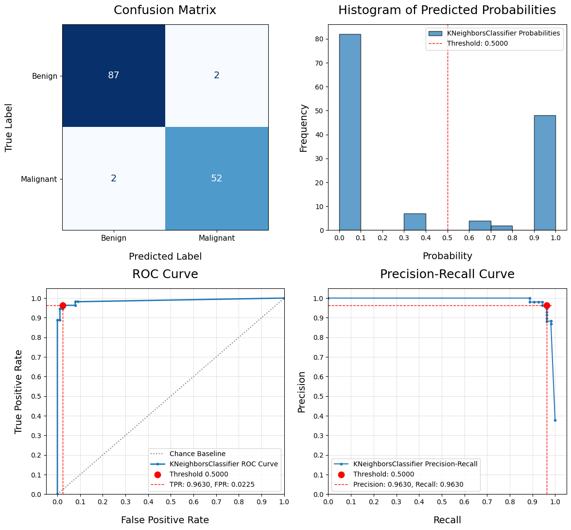
-----------------------------------------------------------------------------------------
3/7: Starting SVC Random Search - May 30, 2024 09:18 AM UTC
-----------------------------------------------------------------------------------------
Fitting 5 folds for each of 10 candidates, totalling 50 fits
[CV 1/5] END svm_proba__C=0.01, svm_proba__kernel=poly;, score=0.756 total time= 0.0s
[CV 2/5] END svm_proba__C=0.01, svm_proba__kernel=poly;, score=0.671 total time= 0.0s
[CV 3/5] END svm_proba__C=0.01, svm_proba__kernel=poly;, score=0.741 total time= 0.0s
[CV 4/5] END svm_proba__C=0.01, svm_proba__kernel=poly;, score=0.635 total time= 0.0s
[CV 5/5] END svm_proba__C=0.01, svm_proba__kernel=poly;, score=0.635 total time= 0.0s
[CV 1/5] END svm_proba__C=100, svm_proba__kernel=poly;, score=0.988 total time= 0.0s
[CV 2/5] END svm_proba__C=100, svm_proba__kernel=poly;, score=0.941 total time= 0.0s
[CV 3/5] END svm_proba__C=100, svm_proba__kernel=poly;, score=0.953 total time= 0.0s
[CV 4/5] END svm_proba__C=100, svm_proba__kernel=poly;, score=0.965 total time= 0.0s
[CV 5/5] END svm_proba__C=100, svm_proba__kernel=poly;, score=0.953 total time= 0.0s
[CV 1/5] END svm_proba__C=0.01, svm_proba__kernel=linear;, score=1.000 total time= 0.0s
[CV 2/5] END svm_proba__C=0.01, svm_proba__kernel=linear;, score=0.906 total time= 0.0s
[CV 3/5] END svm_proba__C=0.01, svm_proba__kernel=linear;, score=1.000 total time= 0.0s
[CV 4/5] END svm_proba__C=0.01, svm_proba__kernel=linear;, score=0.953 total time= 0.0s
[CV 5/5] END svm_proba__C=0.01, svm_proba__kernel=linear;, score=0.965 total time= 0.0s
[CV 1/5] END svm_proba__C=10, svm_proba__kernel=poly;, score=0.988 total time= 0.0s
[CV 2/5] END svm_proba__C=10, svm_proba__kernel=poly;, score=0.882 total time= 0.0s
[CV 3/5] END svm_proba__C=10, svm_proba__kernel=poly;, score=0.988 total time= 0.0s
[CV 4/5] END svm_proba__C=10, svm_proba__kernel=poly;, score=0.953 total time= 0.0s
[CV 5/5] END svm_proba__C=10, svm_proba__kernel=poly;, score=0.941 total time= 0.0s
[CV 1/5] END svm_proba__C=0.0001, svm_proba__kernel=linear;, score=0.721 total time= 0.0s
[CV 2/5] END svm_proba__C=0.0001, svm_proba__kernel=linear;, score=0.612 total time= 0.0s
[CV 3/5] END svm_proba__C=0.0001, svm_proba__kernel=linear;, score=0.682 total time= 0.0s
[CV 4/5] END svm_proba__C=0.0001, svm_proba__kernel=linear;, score=0.588 total time= 0.0s
[CV 5/5] END svm_proba__C=0.0001, svm_proba__kernel=linear;, score=0.565 total time= 0.0s
[CV 1/5] END svm_proba__C=0.1, svm_proba__kernel=linear;, score=1.000 total time= 0.0s
[CV 2/5] END svm_proba__C=0.1, svm_proba__kernel=linear;, score=0.929 total time= 0.0s
[CV 3/5] END svm_proba__C=0.1, svm_proba__kernel=linear;, score=1.000 total time= 0.0s
[CV 4/5] END svm_proba__C=0.1, svm_proba__kernel=linear;, score=0.988 total time= 0.0s
[CV 5/5] END svm_proba__C=0.1, svm_proba__kernel=linear;, score=0.965 total time= 0.0s
[CV 1/5] END svm_proba__C=1, svm_proba__kernel=poly;, score=0.930 total time= 0.0s
[CV 2/5] END svm_proba__C=1, svm_proba__kernel=poly;, score=0.847 total time= 0.0s
[CV 3/5] END svm_proba__C=1, svm_proba__kernel=poly;, score=0.953 total time= 0.0s
[CV 4/5] END svm_proba__C=1, svm_proba__kernel=poly;, score=0.894 total time= 0.0s
[CV 5/5] END svm_proba__C=1, svm_proba__kernel=poly;, score=0.894 total time= 0.0s
[CV 1/5] END svm_proba__C=10, svm_proba__kernel=rbf;, score=1.000 total time= 0.0s
[CV 2/5] END svm_proba__C=10, svm_proba__kernel=rbf;, score=0.965 total time= 0.0s
[CV 3/5] END svm_proba__C=10, svm_proba__kernel=rbf;, score=0.976 total time= 0.0s
[CV 4/5] END svm_proba__C=10, svm_proba__kernel=rbf;, score=0.988 total time= 0.0s
[CV 5/5] END svm_proba__C=10, svm_proba__kernel=rbf;, score=0.965 total time= 0.0s
[CV 1/5] END svm_proba__C=0.01, svm_proba__kernel=sigmoid;, score=0.884 total time= 0.0s
[CV 2/5] END svm_proba__C=0.01, svm_proba__kernel=sigmoid;, score=0.776 total time= 0.0s
[CV 3/5] END svm_proba__C=0.01, svm_proba__kernel=sigmoid;, score=0.918 total time= 0.0s
[CV 4/5] END svm_proba__C=0.01, svm_proba__kernel=sigmoid;, score=0.824 total time= 0.0s
[CV 5/5] END svm_proba__C=0.01, svm_proba__kernel=sigmoid;, score=0.812 total time= 0.0s
[CV 1/5] END svm_proba__C=0.1, svm_proba__kernel=poly;, score=0.895 total time= 0.0s
[CV 2/5] END svm_proba__C=0.1, svm_proba__kernel=poly;, score=0.788 total time= 0.0s
[CV 3/5] END svm_proba__C=0.1, svm_proba__kernel=poly;, score=0.894 total time= 0.0s
[CV 4/5] END svm_proba__C=0.1, svm_proba__kernel=poly;, score=0.812 total time= 0.0s
[CV 5/5] END svm_proba__C=0.1, svm_proba__kernel=poly;, score=0.812 total time= 0.0s
Total Time: 1.1188 seconds
Average Fit Time: 0.0224 seconds
Inference Time: 0.0032
Best CV Accuracy Score: 0.9788
Train Accuracy Score: 0.9930
Test Accuracy Score: 0.9650
Overfit: Yes
Overfit Difference: 0.0279
Best Parameters: {'svm_proba__kernel': 'rbf', 'svm_proba__C': 10}
SVC Binary Classification Report
precision recall f1-score support
Benign 0.9773 0.9663 0.9718 89
Malignant 0.9455 0.9630 0.9541 54
accuracy 0.9650 143
macro avg 0.9614 0.9646 0.9629 143
weighted avg 0.9653 0.9650 0.9651 143
ROC AUC: 0.9956
Predicted:0 1
Actual: 0 86 3
Actual: 1 2 52
True Positive Rate / Sensitivity: 0.963
True Negative Rate / Specificity: 0.9663
False Positive Rate / Fall-out: 0.0337
False Negative Rate / Miss Rate: 0.037
Positive Class: Malignant (1)
Threshold: 0.5

-----------------------------------------------------------------------------------------
4/7: Starting DecisionTreeClassifier Random Search - May 30, 2024 09:18 AM UTC
-----------------------------------------------------------------------------------------
Fitting 5 folds for each of 10 candidates, totalling 50 fits
[CV 1/5] END tree_class__criterion=gini, tree_class__max_depth=7, tree_class__min_samples_leaf=2, tree_class__min_samples_split=10;, score=0.965 total time= 0.0s
[CV 2/5] END tree_class__criterion=gini, tree_class__max_depth=7, tree_class__min_samples_leaf=2, tree_class__min_samples_split=10;, score=0.871 total time= 0.1s
[CV 3/5] END tree_class__criterion=gini, tree_class__max_depth=7, tree_class__min_samples_leaf=2, tree_class__min_samples_split=10;, score=0.965 total time= 0.0s
[CV 4/5] END tree_class__criterion=gini, tree_class__max_depth=7, tree_class__min_samples_leaf=2, tree_class__min_samples_split=10;, score=0.941 total time= 0.0s
[CV 5/5] END tree_class__criterion=gini, tree_class__max_depth=7, tree_class__min_samples_leaf=2, tree_class__min_samples_split=10;, score=0.953 total time= 0.0s
[CV 1/5] END tree_class__criterion=entropy, tree_class__max_depth=7, tree_class__min_samples_leaf=4, tree_class__min_samples_split=10;, score=0.907 total time= 0.0s
[CV 2/5] END tree_class__criterion=entropy, tree_class__max_depth=7, tree_class__min_samples_leaf=4, tree_class__min_samples_split=10;, score=0.859 total time= 0.0s
[CV 3/5] END tree_class__criterion=entropy, tree_class__max_depth=7, tree_class__min_samples_leaf=4, tree_class__min_samples_split=10;, score=0.988 total time= 0.0s
[CV 4/5] END tree_class__criterion=entropy, tree_class__max_depth=7, tree_class__min_samples_leaf=4, tree_class__min_samples_split=10;, score=0.941 total time= 0.0s
[CV 5/5] END tree_class__criterion=entropy, tree_class__max_depth=7, tree_class__min_samples_leaf=4, tree_class__min_samples_split=10;, score=0.918 total time= 0.0s
[CV 1/5] END tree_class__criterion=entropy, tree_class__max_depth=7, tree_class__min_samples_leaf=4, tree_class__min_samples_split=5;, score=0.895 total time= 0.0s
[CV 2/5] END tree_class__criterion=entropy, tree_class__max_depth=7, tree_class__min_samples_leaf=4, tree_class__min_samples_split=5;, score=0.882 total time= 0.0s
[CV 3/5] END tree_class__criterion=entropy, tree_class__max_depth=7, tree_class__min_samples_leaf=4, tree_class__min_samples_split=5;, score=0.988 total time= 0.0s
[CV 4/5] END tree_class__criterion=entropy, tree_class__max_depth=7, tree_class__min_samples_leaf=4, tree_class__min_samples_split=5;, score=0.941 total time= 0.0s
[CV 5/5] END tree_class__criterion=entropy, tree_class__max_depth=7, tree_class__min_samples_leaf=4, tree_class__min_samples_split=5;, score=0.918 total time= 0.0s
[CV 1/5] END tree_class__criterion=gini, tree_class__max_depth=5, tree_class__min_samples_leaf=4, tree_class__min_samples_split=5;, score=0.953 total time= 0.0s
[CV 2/5] END tree_class__criterion=gini, tree_class__max_depth=5, tree_class__min_samples_leaf=4, tree_class__min_samples_split=5;, score=0.871 total time= 0.0s
[CV 3/5] END tree_class__criterion=gini, tree_class__max_depth=5, tree_class__min_samples_leaf=4, tree_class__min_samples_split=5;, score=0.976 total time= 0.0s
[CV 4/5] END tree_class__criterion=gini, tree_class__max_depth=5, tree_class__min_samples_leaf=4, tree_class__min_samples_split=5;, score=0.941 total time= 0.0s
[CV 5/5] END tree_class__criterion=gini, tree_class__max_depth=5, tree_class__min_samples_leaf=4, tree_class__min_samples_split=5;, score=0.929 total time= 0.0s
[CV 1/5] END tree_class__criterion=entropy, tree_class__max_depth=5, tree_class__min_samples_leaf=6, tree_class__min_samples_split=15;, score=0.930 total time= 0.0s
[CV 2/5] END tree_class__criterion=entropy, tree_class__max_depth=5, tree_class__min_samples_leaf=6, tree_class__min_samples_split=15;, score=0.859 total time= 0.0s
[CV 3/5] END tree_class__criterion=entropy, tree_class__max_depth=5, tree_class__min_samples_leaf=6, tree_class__min_samples_split=15;, score=1.000 total time= 0.0s
[CV 4/5] END tree_class__criterion=entropy, tree_class__max_depth=5, tree_class__min_samples_leaf=6, tree_class__min_samples_split=15;, score=0.941 total time= 0.0s
[CV 5/5] END tree_class__criterion=entropy, tree_class__max_depth=5, tree_class__min_samples_leaf=6, tree_class__min_samples_split=15;, score=0.894 total time= 0.0s
[CV 1/5] END tree_class__criterion=gini, tree_class__max_depth=3, tree_class__min_samples_leaf=4, tree_class__min_samples_split=15;, score=0.907 total time= 0.0s
[CV 2/5] END tree_class__criterion=gini, tree_class__max_depth=3, tree_class__min_samples_leaf=4, tree_class__min_samples_split=15;, score=0.871 total time= 0.0s
[CV 3/5] END tree_class__criterion=gini, tree_class__max_depth=3, tree_class__min_samples_leaf=4, tree_class__min_samples_split=15;, score=0.988 total time= 0.0s
[CV 4/5] END tree_class__criterion=gini, tree_class__max_depth=3, tree_class__min_samples_leaf=4, tree_class__min_samples_split=15;, score=0.941 total time= 0.0s
[CV 5/5] END tree_class__criterion=gini, tree_class__max_depth=3, tree_class__min_samples_leaf=4, tree_class__min_samples_split=15;, score=0.941 total time= 0.0s
[CV 1/5] END tree_class__criterion=gini, tree_class__max_depth=5, tree_class__min_samples_leaf=6, tree_class__min_samples_split=15;, score=0.907 total time= 0.0s
[CV 2/5] END tree_class__criterion=gini, tree_class__max_depth=5, tree_class__min_samples_leaf=6, tree_class__min_samples_split=15;, score=0.894 total time= 0.0s
[CV 3/5] END tree_class__criterion=gini, tree_class__max_depth=5, tree_class__min_samples_leaf=6, tree_class__min_samples_split=15;, score=0.988 total time= 0.0s
[CV 4/5] END tree_class__criterion=gini, tree_class__max_depth=5, tree_class__min_samples_leaf=6, tree_class__min_samples_split=15;, score=0.941 total time= 0.0s
[CV 5/5] END tree_class__criterion=gini, tree_class__max_depth=5, tree_class__min_samples_leaf=6, tree_class__min_samples_split=15;, score=0.941 total time= 0.0s
[CV 1/5] END tree_class__criterion=entropy, tree_class__max_depth=7, tree_class__min_samples_leaf=6, tree_class__min_samples_split=10;, score=0.907 total time= 0.0s
[CV 2/5] END tree_class__criterion=entropy, tree_class__max_depth=7, tree_class__min_samples_leaf=6, tree_class__min_samples_split=10;, score=0.859 total time= 0.0s
[CV 3/5] END tree_class__criterion=entropy, tree_class__max_depth=7, tree_class__min_samples_leaf=6, tree_class__min_samples_split=10;, score=1.000 total time= 0.0s
[CV 4/5] END tree_class__criterion=entropy, tree_class__max_depth=7, tree_class__min_samples_leaf=6, tree_class__min_samples_split=10;, score=0.941 total time= 0.0s
[CV 5/5] END tree_class__criterion=entropy, tree_class__max_depth=7, tree_class__min_samples_leaf=6, tree_class__min_samples_split=10;, score=0.906 total time= 0.0s
[CV 1/5] END tree_class__criterion=gini, tree_class__max_depth=3, tree_class__min_samples_leaf=4, tree_class__min_samples_split=5;, score=0.965 total time= 0.0s
[CV 2/5] END tree_class__criterion=gini, tree_class__max_depth=3, tree_class__min_samples_leaf=4, tree_class__min_samples_split=5;, score=0.894 total time= 0.0s
[CV 3/5] END tree_class__criterion=gini, tree_class__max_depth=3, tree_class__min_samples_leaf=4, tree_class__min_samples_split=5;, score=0.988 total time= 0.0s
[CV 4/5] END tree_class__criterion=gini, tree_class__max_depth=3, tree_class__min_samples_leaf=4, tree_class__min_samples_split=5;, score=0.941 total time= 0.0s
[CV 5/5] END tree_class__criterion=gini, tree_class__max_depth=3, tree_class__min_samples_leaf=4, tree_class__min_samples_split=5;, score=0.941 total time= 0.0s
[CV 1/5] END tree_class__criterion=entropy, tree_class__max_depth=3, tree_class__min_samples_leaf=4, tree_class__min_samples_split=15;, score=0.930 total time= 0.0s
[CV 2/5] END tree_class__criterion=entropy, tree_class__max_depth=3, tree_class__min_samples_leaf=4, tree_class__min_samples_split=15;, score=0.859 total time= 0.0s
[CV 3/5] END tree_class__criterion=entropy, tree_class__max_depth=3, tree_class__min_samples_leaf=4, tree_class__min_samples_split=15;, score=1.000 total time= 0.0s
[CV 4/5] END tree_class__criterion=entropy, tree_class__max_depth=3, tree_class__min_samples_leaf=4, tree_class__min_samples_split=15;, score=0.941 total time= 0.0s
[CV 5/5] END tree_class__criterion=entropy, tree_class__max_depth=3, tree_class__min_samples_leaf=4, tree_class__min_samples_split=15;, score=0.894 total time= 0.0s
Total Time: 0.5181 seconds
Average Fit Time: 0.0104 seconds
Inference Time: 0.0010
Best CV Accuracy Score: 0.9460
Train Accuracy Score: 0.9695
Test Accuracy Score: 0.9580
Overfit: Yes
Overfit Difference: 0.0114
Best Parameters: {'tree_class__min_samples_split': 5, 'tree_class__min_samples_leaf': 4, 'tree_class__max_depth': 3, 'tree_class__criterion': 'gini'}
DecisionTreeClassifier Binary Classification Report
precision recall f1-score support
Benign 0.9560 0.9775 0.9667 89
Malignant 0.9615 0.9259 0.9434 54
accuracy 0.9580 143
macro avg 0.9588 0.9517 0.9550 143
weighted avg 0.9581 0.9580 0.9579 143
ROC AUC: 0.9526
Predicted:0 1
Actual: 0 87 2
Actual: 1 4 50
True Positive Rate / Sensitivity: 0.9259
True Negative Rate / Specificity: 0.9775
False Positive Rate / Fall-out: 0.0225
False Negative Rate / Miss Rate: 0.0741
Positive Class: Malignant (1)
Threshold: 0.5

-----------------------------------------------------------------------------------------
5/7: Starting RandomForestClassifier Random Search - May 30, 2024 09:18 AM UTC
-----------------------------------------------------------------------------------------
Fitting 5 folds for each of 10 candidates, totalling 50 fits
[CV 1/5] END forest_class__criterion=entropy, forest_class__max_depth=7, forest_class__min_samples_leaf=6, forest_class__min_samples_split=10, forest_class__n_estimators=200;, score=0.942 total time= 0.3s
[CV 2/5] END forest_class__criterion=entropy, forest_class__max_depth=7, forest_class__min_samples_leaf=6, forest_class__min_samples_split=10, forest_class__n_estimators=200;, score=0.929 total time= 0.3s
[CV 3/5] END forest_class__criterion=entropy, forest_class__max_depth=7, forest_class__min_samples_leaf=6, forest_class__min_samples_split=10, forest_class__n_estimators=200;, score=1.000 total time= 0.4s
[CV 4/5] END forest_class__criterion=entropy, forest_class__max_depth=7, forest_class__min_samples_leaf=6, forest_class__min_samples_split=10, forest_class__n_estimators=200;, score=0.976 total time= 0.4s
[CV 5/5] END forest_class__criterion=entropy, forest_class__max_depth=7, forest_class__min_samples_leaf=6, forest_class__min_samples_split=10, forest_class__n_estimators=200;, score=0.941 total time= 0.4s
[CV 1/5] END forest_class__criterion=entropy, forest_class__max_depth=5, forest_class__min_samples_leaf=2, forest_class__min_samples_split=5, forest_class__n_estimators=100;, score=0.942 total time= 0.2s
[CV 2/5] END forest_class__criterion=entropy, forest_class__max_depth=5, forest_class__min_samples_leaf=2, forest_class__min_samples_split=5, forest_class__n_estimators=100;, score=0.929 total time= 0.2s
[CV 3/5] END forest_class__criterion=entropy, forest_class__max_depth=5, forest_class__min_samples_leaf=2, forest_class__min_samples_split=5, forest_class__n_estimators=100;, score=1.000 total time= 0.2s
[CV 4/5] END forest_class__criterion=entropy, forest_class__max_depth=5, forest_class__min_samples_leaf=2, forest_class__min_samples_split=5, forest_class__n_estimators=100;, score=0.976 total time= 0.2s
[CV 5/5] END forest_class__criterion=entropy, forest_class__max_depth=5, forest_class__min_samples_leaf=2, forest_class__min_samples_split=5, forest_class__n_estimators=100;, score=0.965 total time= 0.2s
[CV 1/5] END forest_class__criterion=entropy, forest_class__max_depth=5, forest_class__min_samples_leaf=6, forest_class__min_samples_split=10, forest_class__n_estimators=200;, score=0.942 total time= 0.4s
[CV 2/5] END forest_class__criterion=entropy, forest_class__max_depth=5, forest_class__min_samples_leaf=6, forest_class__min_samples_split=10, forest_class__n_estimators=200;, score=0.918 total time= 0.4s
[CV 3/5] END forest_class__criterion=entropy, forest_class__max_depth=5, forest_class__min_samples_leaf=6, forest_class__min_samples_split=10, forest_class__n_estimators=200;, score=1.000 total time= 0.3s
[CV 4/5] END forest_class__criterion=entropy, forest_class__max_depth=5, forest_class__min_samples_leaf=6, forest_class__min_samples_split=10, forest_class__n_estimators=200;, score=0.976 total time= 0.3s
[CV 5/5] END forest_class__criterion=entropy, forest_class__max_depth=5, forest_class__min_samples_leaf=6, forest_class__min_samples_split=10, forest_class__n_estimators=200;, score=0.929 total time= 0.4s
[CV 1/5] END forest_class__criterion=gini, forest_class__max_depth=7, forest_class__min_samples_leaf=2, forest_class__min_samples_split=5, forest_class__n_estimators=100;, score=0.953 total time= 0.2s
[CV 2/5] END forest_class__criterion=gini, forest_class__max_depth=7, forest_class__min_samples_leaf=2, forest_class__min_samples_split=5, forest_class__n_estimators=100;, score=0.929 total time= 0.2s
[CV 3/5] END forest_class__criterion=gini, forest_class__max_depth=7, forest_class__min_samples_leaf=2, forest_class__min_samples_split=5, forest_class__n_estimators=100;, score=1.000 total time= 0.2s
[CV 4/5] END forest_class__criterion=gini, forest_class__max_depth=7, forest_class__min_samples_leaf=2, forest_class__min_samples_split=5, forest_class__n_estimators=100;, score=0.965 total time= 0.2s
[CV 5/5] END forest_class__criterion=gini, forest_class__max_depth=7, forest_class__min_samples_leaf=2, forest_class__min_samples_split=5, forest_class__n_estimators=100;, score=0.918 total time= 0.2s
[CV 1/5] END forest_class__criterion=entropy, forest_class__max_depth=3, forest_class__min_samples_leaf=4, forest_class__min_samples_split=10, forest_class__n_estimators=100;, score=0.930 total time= 0.2s
[CV 2/5] END forest_class__criterion=entropy, forest_class__max_depth=3, forest_class__min_samples_leaf=4, forest_class__min_samples_split=10, forest_class__n_estimators=100;, score=0.918 total time= 0.2s
[CV 3/5] END forest_class__criterion=entropy, forest_class__max_depth=3, forest_class__min_samples_leaf=4, forest_class__min_samples_split=10, forest_class__n_estimators=100;, score=1.000 total time= 0.2s
[CV 4/5] END forest_class__criterion=entropy, forest_class__max_depth=3, forest_class__min_samples_leaf=4, forest_class__min_samples_split=10, forest_class__n_estimators=100;, score=0.965 total time= 0.2s
[CV 5/5] END forest_class__criterion=entropy, forest_class__max_depth=3, forest_class__min_samples_leaf=4, forest_class__min_samples_split=10, forest_class__n_estimators=100;, score=0.918 total time= 0.2s
[CV 1/5] END forest_class__criterion=gini, forest_class__max_depth=5, forest_class__min_samples_leaf=2, forest_class__min_samples_split=5, forest_class__n_estimators=200;, score=0.942 total time= 0.4s
[CV 2/5] END forest_class__criterion=gini, forest_class__max_depth=5, forest_class__min_samples_leaf=2, forest_class__min_samples_split=5, forest_class__n_estimators=200;, score=0.929 total time= 0.3s
[CV 3/5] END forest_class__criterion=gini, forest_class__max_depth=5, forest_class__min_samples_leaf=2, forest_class__min_samples_split=5, forest_class__n_estimators=200;, score=1.000 total time= 0.4s
[CV 4/5] END forest_class__criterion=gini, forest_class__max_depth=5, forest_class__min_samples_leaf=2, forest_class__min_samples_split=5, forest_class__n_estimators=200;, score=0.976 total time= 0.3s
[CV 5/5] END forest_class__criterion=gini, forest_class__max_depth=5, forest_class__min_samples_leaf=2, forest_class__min_samples_split=5, forest_class__n_estimators=200;, score=0.929 total time= 0.4s
[CV 1/5] END forest_class__criterion=entropy, forest_class__max_depth=3, forest_class__min_samples_leaf=6, forest_class__min_samples_split=5, forest_class__n_estimators=200;, score=0.930 total time= 0.3s
[CV 2/5] END forest_class__criterion=entropy, forest_class__max_depth=3, forest_class__min_samples_leaf=6, forest_class__min_samples_split=5, forest_class__n_estimators=200;, score=0.941 total time= 0.3s
[CV 3/5] END forest_class__criterion=entropy, forest_class__max_depth=3, forest_class__min_samples_leaf=6, forest_class__min_samples_split=5, forest_class__n_estimators=200;, score=1.000 total time= 0.4s
[CV 4/5] END forest_class__criterion=entropy, forest_class__max_depth=3, forest_class__min_samples_leaf=6, forest_class__min_samples_split=5, forest_class__n_estimators=200;, score=0.965 total time= 0.4s
[CV 5/5] END forest_class__criterion=entropy, forest_class__max_depth=3, forest_class__min_samples_leaf=6, forest_class__min_samples_split=5, forest_class__n_estimators=200;, score=0.929 total time= 0.3s
[CV 1/5] END forest_class__criterion=gini, forest_class__max_depth=5, forest_class__min_samples_leaf=6, forest_class__min_samples_split=15, forest_class__n_estimators=50;, score=0.953 total time= 0.1s
[CV 2/5] END forest_class__criterion=gini, forest_class__max_depth=5, forest_class__min_samples_leaf=6, forest_class__min_samples_split=15, forest_class__n_estimators=50;, score=0.929 total time= 0.1s
[CV 3/5] END forest_class__criterion=gini, forest_class__max_depth=5, forest_class__min_samples_leaf=6, forest_class__min_samples_split=15, forest_class__n_estimators=50;, score=1.000 total time= 0.1s
[CV 4/5] END forest_class__criterion=gini, forest_class__max_depth=5, forest_class__min_samples_leaf=6, forest_class__min_samples_split=15, forest_class__n_estimators=50;, score=0.965 total time= 0.1s
[CV 5/5] END forest_class__criterion=gini, forest_class__max_depth=5, forest_class__min_samples_leaf=6, forest_class__min_samples_split=15, forest_class__n_estimators=50;, score=0.918 total time= 0.1s
[CV 1/5] END forest_class__criterion=entropy, forest_class__max_depth=3, forest_class__min_samples_leaf=6, forest_class__min_samples_split=5, forest_class__n_estimators=100;, score=0.930 total time= 0.3s
[CV 2/5] END forest_class__criterion=entropy, forest_class__max_depth=3, forest_class__min_samples_leaf=6, forest_class__min_samples_split=5, forest_class__n_estimators=100;, score=0.929 total time= 0.2s
[CV 3/5] END forest_class__criterion=entropy, forest_class__max_depth=3, forest_class__min_samples_leaf=6, forest_class__min_samples_split=5, forest_class__n_estimators=100;, score=1.000 total time= 0.2s
[CV 4/5] END forest_class__criterion=entropy, forest_class__max_depth=3, forest_class__min_samples_leaf=6, forest_class__min_samples_split=5, forest_class__n_estimators=100;, score=0.965 total time= 0.2s
[CV 5/5] END forest_class__criterion=entropy, forest_class__max_depth=3, forest_class__min_samples_leaf=6, forest_class__min_samples_split=5, forest_class__n_estimators=100;, score=0.918 total time= 0.2s
[CV 1/5] END forest_class__criterion=entropy, forest_class__max_depth=7, forest_class__min_samples_leaf=4, forest_class__min_samples_split=5, forest_class__n_estimators=50;, score=0.953 total time= 0.1s
[CV 2/5] END forest_class__criterion=entropy, forest_class__max_depth=7, forest_class__min_samples_leaf=4, forest_class__min_samples_split=5, forest_class__n_estimators=50;, score=0.918 total time= 0.1s
[CV 3/5] END forest_class__criterion=entropy, forest_class__max_depth=7, forest_class__min_samples_leaf=4, forest_class__min_samples_split=5, forest_class__n_estimators=50;, score=1.000 total time= 0.1s
[CV 4/5] END forest_class__criterion=entropy, forest_class__max_depth=7, forest_class__min_samples_leaf=4, forest_class__min_samples_split=5, forest_class__n_estimators=50;, score=0.976 total time= 0.1s
[CV 5/5] END forest_class__criterion=entropy, forest_class__max_depth=7, forest_class__min_samples_leaf=4, forest_class__min_samples_split=5, forest_class__n_estimators=50;, score=0.941 total time= 0.1s
Total Time: 11.8924 seconds
Average Fit Time: 0.2378 seconds
Inference Time: 0.0064
Best CV Accuracy Score: 0.9625
Train Accuracy Score: 0.9930
Test Accuracy Score: 0.9720
Overfit: Yes
Overfit Difference: 0.0209
Best Parameters: {'forest_class__n_estimators': 100, 'forest_class__min_samples_split': 5, 'forest_class__min_samples_leaf': 2, 'forest_class__max_depth': 5, 'forest_class__criterion': 'entropy'}
RandomForestClassifier Binary Classification Report
precision recall f1-score support
Benign 0.9670 0.9888 0.9778 89
Malignant 0.9808 0.9444 0.9623 54
accuracy 0.9720 143
macro avg 0.9739 0.9666 0.9700 143
weighted avg 0.9722 0.9720 0.9719 143
ROC AUC: 0.9971
Predicted:0 1
Actual: 0 88 1
Actual: 1 3 51
True Positive Rate / Sensitivity: 0.9444
True Negative Rate / Specificity: 0.9888
False Positive Rate / Fall-out: 0.0112
False Negative Rate / Miss Rate: 0.0556
Positive Class: Malignant (1)
Threshold: 0.5
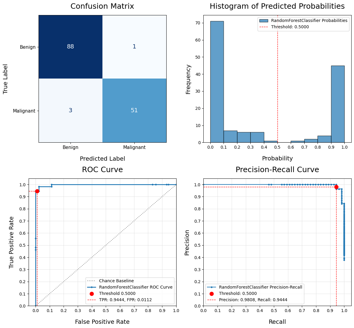
-----------------------------------------------------------------------------------------
6/7: Starting XGBClassifier Random Search - May 30, 2024 09:19 AM UTC
-----------------------------------------------------------------------------------------
Fitting 5 folds for each of 10 candidates, totalling 50 fits
[CV 1/5] END xgb_class__colsample_bytree=0.9, xgb_class__gamma=1, xgb_class__learning_rate=0.1, xgb_class__max_depth=5, xgb_class__n_estimators=50, xgb_class__objective=binary:logistic, xgb_class__subsample=0.9;, score=0.965 total time= 0.1s
[CV 2/5] END xgb_class__colsample_bytree=0.9, xgb_class__gamma=1, xgb_class__learning_rate=0.1, xgb_class__max_depth=5, xgb_class__n_estimators=50, xgb_class__objective=binary:logistic, xgb_class__subsample=0.9;, score=0.906 total time= 0.1s
[CV 3/5] END xgb_class__colsample_bytree=0.9, xgb_class__gamma=1, xgb_class__learning_rate=0.1, xgb_class__max_depth=5, xgb_class__n_estimators=50, xgb_class__objective=binary:logistic, xgb_class__subsample=0.9;, score=1.000 total time= 0.1s
[CV 4/5] END xgb_class__colsample_bytree=0.9, xgb_class__gamma=1, xgb_class__learning_rate=0.1, xgb_class__max_depth=5, xgb_class__n_estimators=50, xgb_class__objective=binary:logistic, xgb_class__subsample=0.9;, score=0.976 total time= 0.1s
[CV 5/5] END xgb_class__colsample_bytree=0.9, xgb_class__gamma=1, xgb_class__learning_rate=0.1, xgb_class__max_depth=5, xgb_class__n_estimators=50, xgb_class__objective=binary:logistic, xgb_class__subsample=0.9;, score=0.953 total time= 0.1s
[CV 1/5] END xgb_class__colsample_bytree=0.7, xgb_class__gamma=0, xgb_class__learning_rate=0.5, xgb_class__max_depth=5, xgb_class__n_estimators=200, xgb_class__objective=binary:logistic, xgb_class__subsample=0.8;, score=0.965 total time= 0.1s
[CV 2/5] END xgb_class__colsample_bytree=0.7, xgb_class__gamma=0, xgb_class__learning_rate=0.5, xgb_class__max_depth=5, xgb_class__n_estimators=200, xgb_class__objective=binary:logistic, xgb_class__subsample=0.8;, score=0.941 total time= 0.1s
[CV 3/5] END xgb_class__colsample_bytree=0.7, xgb_class__gamma=0, xgb_class__learning_rate=0.5, xgb_class__max_depth=5, xgb_class__n_estimators=200, xgb_class__objective=binary:logistic, xgb_class__subsample=0.8;, score=1.000 total time= 0.2s
[CV 4/5] END xgb_class__colsample_bytree=0.7, xgb_class__gamma=0, xgb_class__learning_rate=0.5, xgb_class__max_depth=5, xgb_class__n_estimators=200, xgb_class__objective=binary:logistic, xgb_class__subsample=0.8;, score=0.965 total time= 0.2s
[CV 5/5] END xgb_class__colsample_bytree=0.7, xgb_class__gamma=0, xgb_class__learning_rate=0.5, xgb_class__max_depth=5, xgb_class__n_estimators=200, xgb_class__objective=binary:logistic, xgb_class__subsample=0.8;, score=0.965 total time= 0.1s
[CV 1/5] END xgb_class__colsample_bytree=0.9, xgb_class__gamma=5, xgb_class__learning_rate=0.1, xgb_class__max_depth=7, xgb_class__n_estimators=50, xgb_class__objective=binary:logistic, xgb_class__subsample=0.7;, score=0.953 total time= 0.1s
[CV 2/5] END xgb_class__colsample_bytree=0.9, xgb_class__gamma=5, xgb_class__learning_rate=0.1, xgb_class__max_depth=7, xgb_class__n_estimators=50, xgb_class__objective=binary:logistic, xgb_class__subsample=0.7;, score=0.906 total time= 0.1s
[CV 3/5] END xgb_class__colsample_bytree=0.9, xgb_class__gamma=5, xgb_class__learning_rate=0.1, xgb_class__max_depth=7, xgb_class__n_estimators=50, xgb_class__objective=binary:logistic, xgb_class__subsample=0.7;, score=1.000 total time= 0.1s
[CV 4/5] END xgb_class__colsample_bytree=0.9, xgb_class__gamma=5, xgb_class__learning_rate=0.1, xgb_class__max_depth=7, xgb_class__n_estimators=50, xgb_class__objective=binary:logistic, xgb_class__subsample=0.7;, score=0.965 total time= 0.1s
[CV 5/5] END xgb_class__colsample_bytree=0.9, xgb_class__gamma=5, xgb_class__learning_rate=0.1, xgb_class__max_depth=7, xgb_class__n_estimators=50, xgb_class__objective=binary:logistic, xgb_class__subsample=0.7;, score=0.941 total time= 0.1s
[CV 1/5] END xgb_class__colsample_bytree=0.8, xgb_class__gamma=1, xgb_class__learning_rate=0.5, xgb_class__max_depth=7, xgb_class__n_estimators=200, xgb_class__objective=binary:logistic, xgb_class__subsample=0.9;, score=0.953 total time= 0.1s
[CV 2/5] END xgb_class__colsample_bytree=0.8, xgb_class__gamma=1, xgb_class__learning_rate=0.5, xgb_class__max_depth=7, xgb_class__n_estimators=200, xgb_class__objective=binary:logistic, xgb_class__subsample=0.9;, score=0.929 total time= 0.1s
[CV 3/5] END xgb_class__colsample_bytree=0.8, xgb_class__gamma=1, xgb_class__learning_rate=0.5, xgb_class__max_depth=7, xgb_class__n_estimators=200, xgb_class__objective=binary:logistic, xgb_class__subsample=0.9;, score=1.000 total time= 0.1s
[CV 4/5] END xgb_class__colsample_bytree=0.8, xgb_class__gamma=1, xgb_class__learning_rate=0.5, xgb_class__max_depth=7, xgb_class__n_estimators=200, xgb_class__objective=binary:logistic, xgb_class__subsample=0.9;, score=0.965 total time= 0.1s
[CV 5/5] END xgb_class__colsample_bytree=0.8, xgb_class__gamma=1, xgb_class__learning_rate=0.5, xgb_class__max_depth=7, xgb_class__n_estimators=200, xgb_class__objective=binary:logistic, xgb_class__subsample=0.9;, score=0.953 total time= 0.1s
[CV 1/5] END xgb_class__colsample_bytree=0.8, xgb_class__gamma=10, xgb_class__learning_rate=0.5, xgb_class__max_depth=7, xgb_class__n_estimators=100, xgb_class__objective=binary:logistic, xgb_class__subsample=0.9;, score=0.977 total time= 0.1s
[CV 2/5] END xgb_class__colsample_bytree=0.8, xgb_class__gamma=10, xgb_class__learning_rate=0.5, xgb_class__max_depth=7, xgb_class__n_estimators=100, xgb_class__objective=binary:logistic, xgb_class__subsample=0.9;, score=0.929 total time= 0.1s
[CV 3/5] END xgb_class__colsample_bytree=0.8, xgb_class__gamma=10, xgb_class__learning_rate=0.5, xgb_class__max_depth=7, xgb_class__n_estimators=100, xgb_class__objective=binary:logistic, xgb_class__subsample=0.9;, score=1.000 total time= 0.1s
[CV 4/5] END xgb_class__colsample_bytree=0.8, xgb_class__gamma=10, xgb_class__learning_rate=0.5, xgb_class__max_depth=7, xgb_class__n_estimators=100, xgb_class__objective=binary:logistic, xgb_class__subsample=0.9;, score=0.953 total time= 0.1s
[CV 5/5] END xgb_class__colsample_bytree=0.8, xgb_class__gamma=10, xgb_class__learning_rate=0.5, xgb_class__max_depth=7, xgb_class__n_estimators=100, xgb_class__objective=binary:logistic, xgb_class__subsample=0.9;, score=0.941 total time= 0.1s
[CV 1/5] END xgb_class__colsample_bytree=0.8, xgb_class__gamma=5, xgb_class__learning_rate=0.1, xgb_class__max_depth=7, xgb_class__n_estimators=100, xgb_class__objective=binary:logistic, xgb_class__subsample=0.8;, score=0.965 total time= 0.1s
[CV 2/5] END xgb_class__colsample_bytree=0.8, xgb_class__gamma=5, xgb_class__learning_rate=0.1, xgb_class__max_depth=7, xgb_class__n_estimators=100, xgb_class__objective=binary:logistic, xgb_class__subsample=0.8;, score=0.906 total time= 0.1s
[CV 3/5] END xgb_class__colsample_bytree=0.8, xgb_class__gamma=5, xgb_class__learning_rate=0.1, xgb_class__max_depth=7, xgb_class__n_estimators=100, xgb_class__objective=binary:logistic, xgb_class__subsample=0.8;, score=1.000 total time= 0.1s
[CV 4/5] END xgb_class__colsample_bytree=0.8, xgb_class__gamma=5, xgb_class__learning_rate=0.1, xgb_class__max_depth=7, xgb_class__n_estimators=100, xgb_class__objective=binary:logistic, xgb_class__subsample=0.8;, score=0.965 total time= 0.1s
[CV 5/5] END xgb_class__colsample_bytree=0.8, xgb_class__gamma=5, xgb_class__learning_rate=0.1, xgb_class__max_depth=7, xgb_class__n_estimators=100, xgb_class__objective=binary:logistic, xgb_class__subsample=0.8;, score=0.941 total time= 0.1s
[CV 1/5] END xgb_class__colsample_bytree=0.7, xgb_class__gamma=10, xgb_class__learning_rate=0.1, xgb_class__max_depth=3, xgb_class__n_estimators=200, xgb_class__objective=binary:logistic, xgb_class__subsample=0.8;, score=0.942 total time= 0.1s
[CV 2/5] END xgb_class__colsample_bytree=0.7, xgb_class__gamma=10, xgb_class__learning_rate=0.1, xgb_class__max_depth=3, xgb_class__n_estimators=200, xgb_class__objective=binary:logistic, xgb_class__subsample=0.8;, score=0.906 total time= 0.1s
[CV 3/5] END xgb_class__colsample_bytree=0.7, xgb_class__gamma=10, xgb_class__learning_rate=0.1, xgb_class__max_depth=3, xgb_class__n_estimators=200, xgb_class__objective=binary:logistic, xgb_class__subsample=0.8;, score=1.000 total time= 0.1s
[CV 4/5] END xgb_class__colsample_bytree=0.7, xgb_class__gamma=10, xgb_class__learning_rate=0.1, xgb_class__max_depth=3, xgb_class__n_estimators=200, xgb_class__objective=binary:logistic, xgb_class__subsample=0.8;, score=0.965 total time= 0.1s
[CV 5/5] END xgb_class__colsample_bytree=0.7, xgb_class__gamma=10, xgb_class__learning_rate=0.1, xgb_class__max_depth=3, xgb_class__n_estimators=200, xgb_class__objective=binary:logistic, xgb_class__subsample=0.8;, score=0.929 total time= 0.1s
[CV 1/5] END xgb_class__colsample_bytree=0.7, xgb_class__gamma=10, xgb_class__learning_rate=0.1, xgb_class__max_depth=5, xgb_class__n_estimators=50, xgb_class__objective=binary:logistic, xgb_class__subsample=0.8;, score=0.953 total time= 0.1s
[CV 2/5] END xgb_class__colsample_bytree=0.7, xgb_class__gamma=10, xgb_class__learning_rate=0.1, xgb_class__max_depth=5, xgb_class__n_estimators=50, xgb_class__objective=binary:logistic, xgb_class__subsample=0.8;, score=0.906 total time= 0.1s
[CV 3/5] END xgb_class__colsample_bytree=0.7, xgb_class__gamma=10, xgb_class__learning_rate=0.1, xgb_class__max_depth=5, xgb_class__n_estimators=50, xgb_class__objective=binary:logistic, xgb_class__subsample=0.8;, score=1.000 total time= 0.1s
[CV 4/5] END xgb_class__colsample_bytree=0.7, xgb_class__gamma=10, xgb_class__learning_rate=0.1, xgb_class__max_depth=5, xgb_class__n_estimators=50, xgb_class__objective=binary:logistic, xgb_class__subsample=0.8;, score=0.965 total time= 0.1s
[CV 5/5] END xgb_class__colsample_bytree=0.7, xgb_class__gamma=10, xgb_class__learning_rate=0.1, xgb_class__max_depth=5, xgb_class__n_estimators=50, xgb_class__objective=binary:logistic, xgb_class__subsample=0.8;, score=0.929 total time= 0.1s
[CV 1/5] END xgb_class__colsample_bytree=0.9, xgb_class__gamma=10, xgb_class__learning_rate=0.5, xgb_class__max_depth=7, xgb_class__n_estimators=100, xgb_class__objective=binary:logistic, xgb_class__subsample=0.8;, score=0.930 total time= 0.1s
[CV 2/5] END xgb_class__colsample_bytree=0.9, xgb_class__gamma=10, xgb_class__learning_rate=0.5, xgb_class__max_depth=7, xgb_class__n_estimators=100, xgb_class__objective=binary:logistic, xgb_class__subsample=0.8;, score=0.918 total time= 0.1s
[CV 3/5] END xgb_class__colsample_bytree=0.9, xgb_class__gamma=10, xgb_class__learning_rate=0.5, xgb_class__max_depth=7, xgb_class__n_estimators=100, xgb_class__objective=binary:logistic, xgb_class__subsample=0.8;, score=1.000 total time= 0.2s
[CV 4/5] END xgb_class__colsample_bytree=0.9, xgb_class__gamma=10, xgb_class__learning_rate=0.5, xgb_class__max_depth=7, xgb_class__n_estimators=100, xgb_class__objective=binary:logistic, xgb_class__subsample=0.8;, score=0.965 total time= 0.1s
[CV 5/5] END xgb_class__colsample_bytree=0.9, xgb_class__gamma=10, xgb_class__learning_rate=0.5, xgb_class__max_depth=7, xgb_class__n_estimators=100, xgb_class__objective=binary:logistic, xgb_class__subsample=0.8;, score=0.953 total time= 0.1s
[CV 1/5] END xgb_class__colsample_bytree=0.9, xgb_class__gamma=5, xgb_class__learning_rate=0.5, xgb_class__max_depth=7, xgb_class__n_estimators=200, xgb_class__objective=binary:logistic, xgb_class__subsample=0.8;, score=0.942 total time= 0.1s
[CV 2/5] END xgb_class__colsample_bytree=0.9, xgb_class__gamma=5, xgb_class__learning_rate=0.5, xgb_class__max_depth=7, xgb_class__n_estimators=200, xgb_class__objective=binary:logistic, xgb_class__subsample=0.8;, score=0.929 total time= 0.1s
[CV 3/5] END xgb_class__colsample_bytree=0.9, xgb_class__gamma=5, xgb_class__learning_rate=0.5, xgb_class__max_depth=7, xgb_class__n_estimators=200, xgb_class__objective=binary:logistic, xgb_class__subsample=0.8;, score=1.000 total time= 0.2s
[CV 4/5] END xgb_class__colsample_bytree=0.9, xgb_class__gamma=5, xgb_class__learning_rate=0.5, xgb_class__max_depth=7, xgb_class__n_estimators=200, xgb_class__objective=binary:logistic, xgb_class__subsample=0.8;, score=0.976 total time= 0.1s
[CV 5/5] END xgb_class__colsample_bytree=0.9, xgb_class__gamma=5, xgb_class__learning_rate=0.5, xgb_class__max_depth=7, xgb_class__n_estimators=200, xgb_class__objective=binary:logistic, xgb_class__subsample=0.8;, score=0.953 total time= 0.1s
Total Time: 5.5002 seconds
Average Fit Time: 0.1100 seconds
Inference Time: 0.0026
Best CV Accuracy Score: 0.9671
Train Accuracy Score: 1.0000
Test Accuracy Score: 0.9580
Overfit: Yes
Overfit Difference: 0.0420
Best Parameters: {'xgb_class__subsample': 0.8, 'xgb_class__objective': 'binary:logistic', 'xgb_class__n_estimators': 200, 'xgb_class__max_depth': 5, 'xgb_class__learning_rate': 0.5, 'xgb_class__gamma': 0, 'xgb_class__colsample_bytree': 0.7}
XGBClassifier Binary Classification Report
precision recall f1-score support
Benign 0.9770 0.9551 0.9659 89
Malignant 0.9286 0.9630 0.9455 54
accuracy 0.9580 143
macro avg 0.9528 0.9590 0.9557 143
weighted avg 0.9587 0.9580 0.9582 143
ROC AUC: 0.9952
Predicted:0 1
Actual: 0 85 4
Actual: 1 2 52
True Positive Rate / Sensitivity: 0.963
True Negative Rate / Specificity: 0.9551
False Positive Rate / Fall-out: 0.0449
False Negative Rate / Miss Rate: 0.037
Positive Class: Malignant (1)
Threshold: 0.5

-----------------------------------------------------------------------------------------
7/7: Starting KerasClassifier Random Search - May 30, 2024 09:19 AM UTC
-----------------------------------------------------------------------------------------
Fitting 5 folds for each of 10 candidates, totalling 50 fits
[CV 1/5] END keras_class__dropout_rate=0.5, keras_class__fit__batch_size=32, keras_class__hidden_layer_dim=50, keras_class__l2_reg=0.0, keras_class__loss=binary_crossentropy, keras_class__optimizer=adam, keras_class__optimizer__learning_rate=0.001, keras_class__second_layer_dim=50, keras_class__third_layer_dim=None;, score=1.000 total time= 3.8s
[CV 2/5] END keras_class__dropout_rate=0.5, keras_class__fit__batch_size=32, keras_class__hidden_layer_dim=50, keras_class__l2_reg=0.0, keras_class__loss=binary_crossentropy, keras_class__optimizer=adam, keras_class__optimizer__learning_rate=0.001, keras_class__second_layer_dim=50, keras_class__third_layer_dim=None;, score=0.929 total time= 3.0s
WARNING:tensorflow:5 out of the last 7 calls to <function TensorFlowTrainer.make_predict_function.<locals>.one_step_on_data_distributed at 0x7fe80a47d430> triggered tf.function retracing. Tracing is expensive and the excessive number of tracings could be due to (1) creating @tf.function repeatedly in a loop, (2) passing tensors with different shapes, (3) passing Python objects instead of tensors. For (1), please define your @tf.function outside of the loop. For (2), @tf.function has reduce_retracing=True option that can avoid unnecessary retracing. For (3), please refer to https://www.tensorflow.org/guide/function#controlling_retracing and https://www.tensorflow.org/api_docs/python/tf/function for more details.
WARNING:tensorflow:6 out of the last 9 calls to <function TensorFlowTrainer.make_predict_function.<locals>.one_step_on_data_distributed at 0x7fe80a47d430> triggered tf.function retracing. Tracing is expensive and the excessive number of tracings could be due to (1) creating @tf.function repeatedly in a loop, (2) passing tensors with different shapes, (3) passing Python objects instead of tensors. For (1), please define your @tf.function outside of the loop. For (2), @tf.function has reduce_retracing=True option that can avoid unnecessary retracing. For (3), please refer to https://www.tensorflow.org/guide/function#controlling_retracing and https://www.tensorflow.org/api_docs/python/tf/function for more details.
[CV 3/5] END keras_class__dropout_rate=0.5, keras_class__fit__batch_size=32, keras_class__hidden_layer_dim=50, keras_class__l2_reg=0.0, keras_class__loss=binary_crossentropy, keras_class__optimizer=adam, keras_class__optimizer__learning_rate=0.001, keras_class__second_layer_dim=50, keras_class__third_layer_dim=None;, score=1.000 total time= 2.9s
[CV 4/5] END keras_class__dropout_rate=0.5, keras_class__fit__batch_size=32, keras_class__hidden_layer_dim=50, keras_class__l2_reg=0.0, keras_class__loss=binary_crossentropy, keras_class__optimizer=adam, keras_class__optimizer__learning_rate=0.001, keras_class__second_layer_dim=50, keras_class__third_layer_dim=None;, score=0.965 total time= 3.8s
[CV 5/5] END keras_class__dropout_rate=0.5, keras_class__fit__batch_size=32, keras_class__hidden_layer_dim=50, keras_class__l2_reg=0.0, keras_class__loss=binary_crossentropy, keras_class__optimizer=adam, keras_class__optimizer__learning_rate=0.001, keras_class__second_layer_dim=50, keras_class__third_layer_dim=None;, score=0.976 total time= 3.3s
[CV 1/5] END keras_class__dropout_rate=0.5, keras_class__fit__batch_size=32, keras_class__hidden_layer_dim=50, keras_class__l2_reg=0.0, keras_class__loss=binary_crossentropy, keras_class__optimizer=adam, keras_class__optimizer__learning_rate=0.001, keras_class__second_layer_dim=50, keras_class__third_layer_dim=25;, score=0.988 total time= 3.4s
[CV 2/5] END keras_class__dropout_rate=0.5, keras_class__fit__batch_size=32, keras_class__hidden_layer_dim=50, keras_class__l2_reg=0.0, keras_class__loss=binary_crossentropy, keras_class__optimizer=adam, keras_class__optimizer__learning_rate=0.001, keras_class__second_layer_dim=50, keras_class__third_layer_dim=25;, score=0.918 total time= 4.4s
[CV 3/5] END keras_class__dropout_rate=0.5, keras_class__fit__batch_size=32, keras_class__hidden_layer_dim=50, keras_class__l2_reg=0.0, keras_class__loss=binary_crossentropy, keras_class__optimizer=adam, keras_class__optimizer__learning_rate=0.001, keras_class__second_layer_dim=50, keras_class__third_layer_dim=25;, score=1.000 total time= 3.7s
[CV 4/5] END keras_class__dropout_rate=0.5, keras_class__fit__batch_size=32, keras_class__hidden_layer_dim=50, keras_class__l2_reg=0.0, keras_class__loss=binary_crossentropy, keras_class__optimizer=adam, keras_class__optimizer__learning_rate=0.001, keras_class__second_layer_dim=50, keras_class__third_layer_dim=25;, score=0.976 total time= 5.0s
[CV 5/5] END keras_class__dropout_rate=0.5, keras_class__fit__batch_size=32, keras_class__hidden_layer_dim=50, keras_class__l2_reg=0.0, keras_class__loss=binary_crossentropy, keras_class__optimizer=adam, keras_class__optimizer__learning_rate=0.001, keras_class__second_layer_dim=50, keras_class__third_layer_dim=25;, score=0.965 total time= 4.6s
[CV 1/5] END keras_class__dropout_rate=0.5, keras_class__fit__batch_size=32, keras_class__hidden_layer_dim=100, keras_class__l2_reg=0.0, keras_class__loss=binary_crossentropy, keras_class__optimizer=adam, keras_class__optimizer__learning_rate=0.001, keras_class__second_layer_dim=50, keras_class__third_layer_dim=50;, score=1.000 total time= 4.1s
[CV 2/5] END keras_class__dropout_rate=0.5, keras_class__fit__batch_size=32, keras_class__hidden_layer_dim=100, keras_class__l2_reg=0.0, keras_class__loss=binary_crossentropy, keras_class__optimizer=adam, keras_class__optimizer__learning_rate=0.001, keras_class__second_layer_dim=50, keras_class__third_layer_dim=50;, score=0.918 total time= 3.7s
[CV 3/5] END keras_class__dropout_rate=0.5, keras_class__fit__batch_size=32, keras_class__hidden_layer_dim=100, keras_class__l2_reg=0.0, keras_class__loss=binary_crossentropy, keras_class__optimizer=adam, keras_class__optimizer__learning_rate=0.001, keras_class__second_layer_dim=50, keras_class__third_layer_dim=50;, score=1.000 total time= 3.2s
[CV 4/5] END keras_class__dropout_rate=0.5, keras_class__fit__batch_size=32, keras_class__hidden_layer_dim=100, keras_class__l2_reg=0.0, keras_class__loss=binary_crossentropy, keras_class__optimizer=adam, keras_class__optimizer__learning_rate=0.001, keras_class__second_layer_dim=50, keras_class__third_layer_dim=50;, score=0.976 total time= 3.7s
[CV 5/5] END keras_class__dropout_rate=0.5, keras_class__fit__batch_size=32, keras_class__hidden_layer_dim=100, keras_class__l2_reg=0.0, keras_class__loss=binary_crossentropy, keras_class__optimizer=adam, keras_class__optimizer__learning_rate=0.001, keras_class__second_layer_dim=50, keras_class__third_layer_dim=50;, score=0.965 total time= 3.9s
[CV 1/5] END keras_class__dropout_rate=0.5, keras_class__fit__batch_size=32, keras_class__hidden_layer_dim=50, keras_class__l2_reg=0.0, keras_class__loss=binary_crossentropy, keras_class__optimizer=adam, keras_class__optimizer__learning_rate=0.001, keras_class__second_layer_dim=100, keras_class__third_layer_dim=50;, score=0.988 total time= 3.4s
[CV 2/5] END keras_class__dropout_rate=0.5, keras_class__fit__batch_size=32, keras_class__hidden_layer_dim=50, keras_class__l2_reg=0.0, keras_class__loss=binary_crossentropy, keras_class__optimizer=adam, keras_class__optimizer__learning_rate=0.001, keras_class__second_layer_dim=100, keras_class__third_layer_dim=50;, score=0.929 total time= 2.9s
[CV 3/5] END keras_class__dropout_rate=0.5, keras_class__fit__batch_size=32, keras_class__hidden_layer_dim=50, keras_class__l2_reg=0.0, keras_class__loss=binary_crossentropy, keras_class__optimizer=adam, keras_class__optimizer__learning_rate=0.001, keras_class__second_layer_dim=100, keras_class__third_layer_dim=50;, score=1.000 total time= 2.7s
[CV 4/5] END keras_class__dropout_rate=0.5, keras_class__fit__batch_size=32, keras_class__hidden_layer_dim=50, keras_class__l2_reg=0.0, keras_class__loss=binary_crossentropy, keras_class__optimizer=adam, keras_class__optimizer__learning_rate=0.001, keras_class__second_layer_dim=100, keras_class__third_layer_dim=50;, score=0.976 total time= 6.6s
[CV 5/5] END keras_class__dropout_rate=0.5, keras_class__fit__batch_size=32, keras_class__hidden_layer_dim=50, keras_class__l2_reg=0.0, keras_class__loss=binary_crossentropy, keras_class__optimizer=adam, keras_class__optimizer__learning_rate=0.001, keras_class__second_layer_dim=100, keras_class__third_layer_dim=50;, score=0.965 total time= 4.8s
[CV 1/5] END keras_class__dropout_rate=0.5, keras_class__fit__batch_size=32, keras_class__hidden_layer_dim=50, keras_class__l2_reg=0.0, keras_class__loss=binary_crossentropy, keras_class__optimizer=adam, keras_class__optimizer__learning_rate=0.001, keras_class__second_layer_dim=100, keras_class__third_layer_dim=None;, score=1.000 total time= 3.4s
[CV 2/5] END keras_class__dropout_rate=0.5, keras_class__fit__batch_size=32, keras_class__hidden_layer_dim=50, keras_class__l2_reg=0.0, keras_class__loss=binary_crossentropy, keras_class__optimizer=adam, keras_class__optimizer__learning_rate=0.001, keras_class__second_layer_dim=100, keras_class__third_layer_dim=None;, score=0.929 total time= 3.8s
[CV 3/5] END keras_class__dropout_rate=0.5, keras_class__fit__batch_size=32, keras_class__hidden_layer_dim=50, keras_class__l2_reg=0.0, keras_class__loss=binary_crossentropy, keras_class__optimizer=adam, keras_class__optimizer__learning_rate=0.001, keras_class__second_layer_dim=100, keras_class__third_layer_dim=None;, score=1.000 total time= 3.6s
[CV 4/5] END keras_class__dropout_rate=0.5, keras_class__fit__batch_size=32, keras_class__hidden_layer_dim=50, keras_class__l2_reg=0.0, keras_class__loss=binary_crossentropy, keras_class__optimizer=adam, keras_class__optimizer__learning_rate=0.001, keras_class__second_layer_dim=100, keras_class__third_layer_dim=None;, score=0.988 total time= 4.0s
[CV 5/5] END keras_class__dropout_rate=0.5, keras_class__fit__batch_size=32, keras_class__hidden_layer_dim=50, keras_class__l2_reg=0.0, keras_class__loss=binary_crossentropy, keras_class__optimizer=adam, keras_class__optimizer__learning_rate=0.001, keras_class__second_layer_dim=100, keras_class__third_layer_dim=None;, score=0.976 total time= 3.3s
[CV 1/5] END keras_class__dropout_rate=0.5, keras_class__fit__batch_size=32, keras_class__hidden_layer_dim=200, keras_class__l2_reg=0.0, keras_class__loss=binary_crossentropy, keras_class__optimizer=adam, keras_class__optimizer__learning_rate=0.001, keras_class__second_layer_dim=50, keras_class__third_layer_dim=25;, score=1.000 total time= 2.7s
[CV 2/5] END keras_class__dropout_rate=0.5, keras_class__fit__batch_size=32, keras_class__hidden_layer_dim=200, keras_class__l2_reg=0.0, keras_class__loss=binary_crossentropy, keras_class__optimizer=adam, keras_class__optimizer__learning_rate=0.001, keras_class__second_layer_dim=50, keras_class__third_layer_dim=25;, score=0.929 total time= 3.0s
[CV 3/5] END keras_class__dropout_rate=0.5, keras_class__fit__batch_size=32, keras_class__hidden_layer_dim=200, keras_class__l2_reg=0.0, keras_class__loss=binary_crossentropy, keras_class__optimizer=adam, keras_class__optimizer__learning_rate=0.001, keras_class__second_layer_dim=50, keras_class__third_layer_dim=25;, score=1.000 total time= 3.5s
[CV 4/5] END keras_class__dropout_rate=0.5, keras_class__fit__batch_size=32, keras_class__hidden_layer_dim=200, keras_class__l2_reg=0.0, keras_class__loss=binary_crossentropy, keras_class__optimizer=adam, keras_class__optimizer__learning_rate=0.001, keras_class__second_layer_dim=50, keras_class__third_layer_dim=25;, score=0.976 total time= 4.7s
[CV 5/5] END keras_class__dropout_rate=0.5, keras_class__fit__batch_size=32, keras_class__hidden_layer_dim=200, keras_class__l2_reg=0.0, keras_class__loss=binary_crossentropy, keras_class__optimizer=adam, keras_class__optimizer__learning_rate=0.001, keras_class__second_layer_dim=50, keras_class__third_layer_dim=25;, score=0.965 total time= 5.1s
[CV 1/5] END keras_class__dropout_rate=0.5, keras_class__fit__batch_size=32, keras_class__hidden_layer_dim=200, keras_class__l2_reg=0.0, keras_class__loss=binary_crossentropy, keras_class__optimizer=adam, keras_class__optimizer__learning_rate=0.001, keras_class__second_layer_dim=100, keras_class__third_layer_dim=25;, score=1.000 total time= 2.8s
[CV 2/5] END keras_class__dropout_rate=0.5, keras_class__fit__batch_size=32, keras_class__hidden_layer_dim=200, keras_class__l2_reg=0.0, keras_class__loss=binary_crossentropy, keras_class__optimizer=adam, keras_class__optimizer__learning_rate=0.001, keras_class__second_layer_dim=100, keras_class__third_layer_dim=25;, score=0.929 total time= 3.1s
[CV 3/5] END keras_class__dropout_rate=0.5, keras_class__fit__batch_size=32, keras_class__hidden_layer_dim=200, keras_class__l2_reg=0.0, keras_class__loss=binary_crossentropy, keras_class__optimizer=adam, keras_class__optimizer__learning_rate=0.001, keras_class__second_layer_dim=100, keras_class__third_layer_dim=25;, score=1.000 total time= 2.7s
[CV 4/5] END keras_class__dropout_rate=0.5, keras_class__fit__batch_size=32, keras_class__hidden_layer_dim=200, keras_class__l2_reg=0.0, keras_class__loss=binary_crossentropy, keras_class__optimizer=adam, keras_class__optimizer__learning_rate=0.001, keras_class__second_layer_dim=100, keras_class__third_layer_dim=25;, score=0.976 total time= 3.7s
[CV 5/5] END keras_class__dropout_rate=0.5, keras_class__fit__batch_size=32, keras_class__hidden_layer_dim=200, keras_class__l2_reg=0.0, keras_class__loss=binary_crossentropy, keras_class__optimizer=adam, keras_class__optimizer__learning_rate=0.001, keras_class__second_layer_dim=100, keras_class__third_layer_dim=25;, score=0.976 total time= 2.7s
[CV 1/5] END keras_class__dropout_rate=0.5, keras_class__fit__batch_size=32, keras_class__hidden_layer_dim=200, keras_class__l2_reg=0.0, keras_class__loss=binary_crossentropy, keras_class__optimizer=adam, keras_class__optimizer__learning_rate=0.001, keras_class__second_layer_dim=100, keras_class__third_layer_dim=None;, score=0.988 total time= 2.1s
[CV 2/5] END keras_class__dropout_rate=0.5, keras_class__fit__batch_size=32, keras_class__hidden_layer_dim=200, keras_class__l2_reg=0.0, keras_class__loss=binary_crossentropy, keras_class__optimizer=adam, keras_class__optimizer__learning_rate=0.001, keras_class__second_layer_dim=100, keras_class__third_layer_dim=None;, score=0.929 total time= 3.4s
[CV 3/5] END keras_class__dropout_rate=0.5, keras_class__fit__batch_size=32, keras_class__hidden_layer_dim=200, keras_class__l2_reg=0.0, keras_class__loss=binary_crossentropy, keras_class__optimizer=adam, keras_class__optimizer__learning_rate=0.001, keras_class__second_layer_dim=100, keras_class__third_layer_dim=None;, score=1.000 total time= 2.7s
[CV 4/5] END keras_class__dropout_rate=0.5, keras_class__fit__batch_size=32, keras_class__hidden_layer_dim=200, keras_class__l2_reg=0.0, keras_class__loss=binary_crossentropy, keras_class__optimizer=adam, keras_class__optimizer__learning_rate=0.001, keras_class__second_layer_dim=100, keras_class__third_layer_dim=None;, score=0.988 total time= 2.9s
[CV 5/5] END keras_class__dropout_rate=0.5, keras_class__fit__batch_size=32, keras_class__hidden_layer_dim=200, keras_class__l2_reg=0.0, keras_class__loss=binary_crossentropy, keras_class__optimizer=adam, keras_class__optimizer__learning_rate=0.001, keras_class__second_layer_dim=100, keras_class__third_layer_dim=None;, score=0.976 total time= 2.3s
[CV 1/5] END keras_class__dropout_rate=0.5, keras_class__fit__batch_size=32, keras_class__hidden_layer_dim=100, keras_class__l2_reg=0.0, keras_class__loss=binary_crossentropy, keras_class__optimizer=adam, keras_class__optimizer__learning_rate=0.001, keras_class__second_layer_dim=100, keras_class__third_layer_dim=50;, score=0.988 total time= 2.7s
[CV 2/5] END keras_class__dropout_rate=0.5, keras_class__fit__batch_size=32, keras_class__hidden_layer_dim=100, keras_class__l2_reg=0.0, keras_class__loss=binary_crossentropy, keras_class__optimizer=adam, keras_class__optimizer__learning_rate=0.001, keras_class__second_layer_dim=100, keras_class__third_layer_dim=50;, score=0.929 total time= 4.9s
[CV 3/5] END keras_class__dropout_rate=0.5, keras_class__fit__batch_size=32, keras_class__hidden_layer_dim=100, keras_class__l2_reg=0.0, keras_class__loss=binary_crossentropy, keras_class__optimizer=adam, keras_class__optimizer__learning_rate=0.001, keras_class__second_layer_dim=100, keras_class__third_layer_dim=50;, score=1.000 total time= 4.8s
[CV 4/5] END keras_class__dropout_rate=0.5, keras_class__fit__batch_size=32, keras_class__hidden_layer_dim=100, keras_class__l2_reg=0.0, keras_class__loss=binary_crossentropy, keras_class__optimizer=adam, keras_class__optimizer__learning_rate=0.001, keras_class__second_layer_dim=100, keras_class__third_layer_dim=50;, score=0.976 total time= 4.0s
[CV 5/5] END keras_class__dropout_rate=0.5, keras_class__fit__batch_size=32, keras_class__hidden_layer_dim=100, keras_class__l2_reg=0.0, keras_class__loss=binary_crossentropy, keras_class__optimizer=adam, keras_class__optimizer__learning_rate=0.001, keras_class__second_layer_dim=100, keras_class__third_layer_dim=50;, score=0.965 total time= 3.6s
[CV 1/5] END keras_class__dropout_rate=0.5, keras_class__fit__batch_size=32, keras_class__hidden_layer_dim=50, keras_class__l2_reg=0.0, keras_class__loss=binary_crossentropy, keras_class__optimizer=adam, keras_class__optimizer__learning_rate=0.001, keras_class__second_layer_dim=50, keras_class__third_layer_dim=50;, score=1.000 total time= 3.5s
[CV 2/5] END keras_class__dropout_rate=0.5, keras_class__fit__batch_size=32, keras_class__hidden_layer_dim=50, keras_class__l2_reg=0.0, keras_class__loss=binary_crossentropy, keras_class__optimizer=adam, keras_class__optimizer__learning_rate=0.001, keras_class__second_layer_dim=50, keras_class__third_layer_dim=50;, score=0.906 total time= 3.9s
[CV 3/5] END keras_class__dropout_rate=0.5, keras_class__fit__batch_size=32, keras_class__hidden_layer_dim=50, keras_class__l2_reg=0.0, keras_class__loss=binary_crossentropy, keras_class__optimizer=adam, keras_class__optimizer__learning_rate=0.001, keras_class__second_layer_dim=50, keras_class__third_layer_dim=50;, score=1.000 total time= 3.9s
[CV 4/5] END keras_class__dropout_rate=0.5, keras_class__fit__batch_size=32, keras_class__hidden_layer_dim=50, keras_class__l2_reg=0.0, keras_class__loss=binary_crossentropy, keras_class__optimizer=adam, keras_class__optimizer__learning_rate=0.001, keras_class__second_layer_dim=50, keras_class__third_layer_dim=50;, score=0.976 total time= 3.8s
[CV 5/5] END keras_class__dropout_rate=0.5, keras_class__fit__batch_size=32, keras_class__hidden_layer_dim=50, keras_class__l2_reg=0.0, keras_class__loss=binary_crossentropy, keras_class__optimizer=adam, keras_class__optimizer__learning_rate=0.001, keras_class__second_layer_dim=50, keras_class__third_layer_dim=50;, score=0.965 total time= 3.3s
Total Time: 183.7382 seconds
Average Fit Time: 3.6748 seconds
Inference Time: 0.0684
Best CV Accuracy Score: 0.9788
Train Accuracy Score: 0.9836
Test Accuracy Score: 0.9790
Overfit: Yes
Overfit Difference: 0.0045
Best Parameters: {'keras_class__third_layer_dim': None, 'keras_class__second_layer_dim': 100, 'keras_class__optimizer__learning_rate': 0.001, 'keras_class__optimizer': 'adam', 'keras_class__loss': 'binary_crossentropy', 'keras_class__l2_reg': 0.0, 'keras_class__hidden_layer_dim': 50, 'keras_class__fit__batch_size': 32, 'keras_class__dropout_rate': 0.5}
Model: "Sequential"
┏━━━━━━━━━━━━━━━━━━━━━━━━━━━━━━━━━┳━━━━━━━━━━━━━━━━━━━━━━━━┳━━━━━━━━━━━━━━━┓ ┃ Layer (type) ┃ Output Shape ┃ Param # ┃ ┡━━━━━━━━━━━━━━━━━━━━━━━━━━━━━━━━━╇━━━━━━━━━━━━━━━━━━━━━━━━╇━━━━━━━━━━━━━━━┩ │ Hidden_1 (Dense) │ (None, 50) │ 1,550 │ ├─────────────────────────────────┼────────────────────────┼───────────────┤ │ Dropout_1 (Dropout) │ (None, 50) │ 0 │ ├─────────────────────────────────┼────────────────────────┼───────────────┤ │ Hidden_2 (Dense) │ (None, 100) │ 5,100 │ ├─────────────────────────────────┼────────────────────────┼───────────────┤ │ Dropout_2 (Dropout) │ (None, 100) │ 0 │ ├─────────────────────────────────┼────────────────────────┼───────────────┤ │ Output (Dense) │ (None, 1) │ 101 │ └─────────────────────────────────┴────────────────────────┴───────────────┘
Total params: 20,255 (79.12 KB)
Trainable params: 6,751 (26.37 KB)
Non-trainable params: 0 (0.00 B)
Optimizer params: 13,504 (52.75 KB)
KerasClassifier Binary Classification Report
precision recall f1-score support
Benign 0.9886 0.9775 0.9831 89
Malignant 0.9636 0.9815 0.9725 54
accuracy 0.9790 143
macro avg 0.9761 0.9795 0.9778 143
weighted avg 0.9792 0.9790 0.9791 143
ROC AUC: 0.9965
Predicted:0 1
Actual: 0 87 2
Actual: 1 1 53
True Positive Rate / Sensitivity: 0.9815
True Negative Rate / Specificity: 0.9775
False Positive Rate / Fall-out: 0.0225
False Negative Rate / Miss Rate: 0.0185
Positive Class: Malignant (1)
Threshold: 0.5
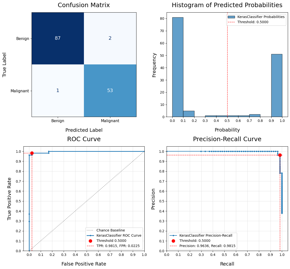
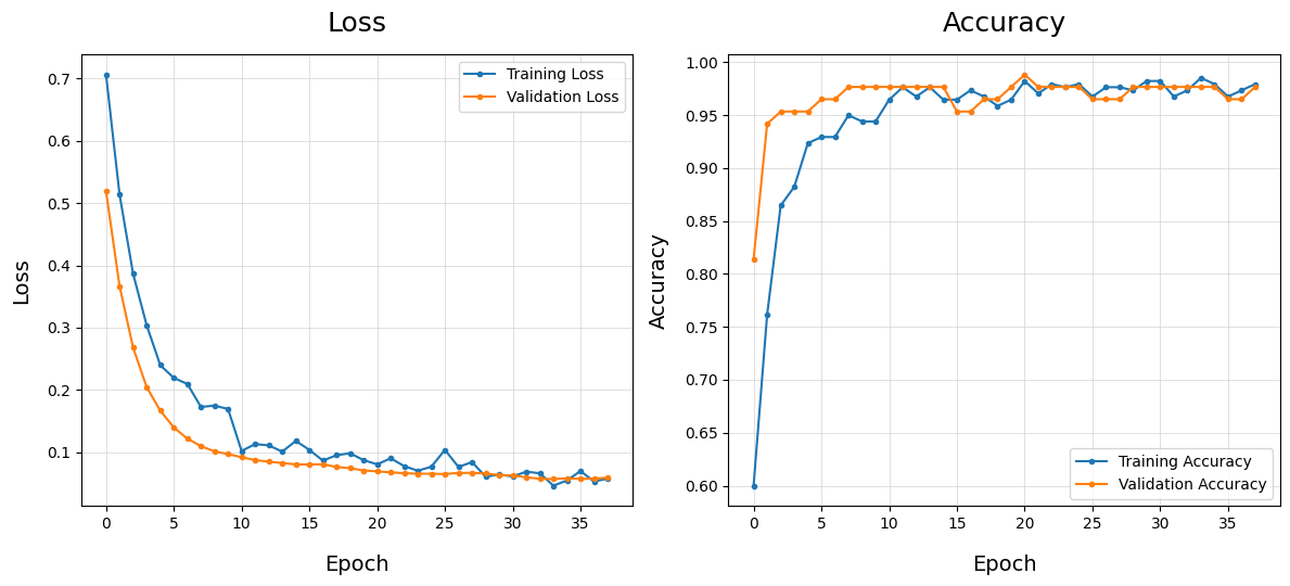
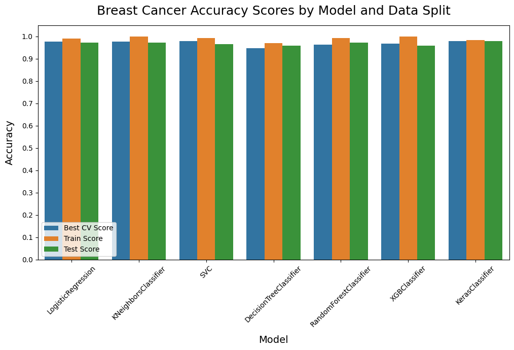
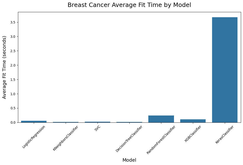
Review the Best Models#
In addition to seeing the charts in the dw.compare_models output, we also have the metrics stored in a dataframe. So we can further analyze or plot the performance of the difference models.
Multiple runs of this function can be stored as different dataframes, with different parameters (ex: varying the X dataset, changing the test size, or using different pre-processing steps in the Pipeline). You can make notes about these differences in the notes parameter. Then multiple dataframes can be concatenated and evaluate as one.
[143]:
# Review the results
results_df
[143]:
| Model | Test Size | Over Sample | Under Sample | Resample | Total Fit Time | Fit Count | Average Fit Time | Inference Time | Grid Scorer | Best Params | Best CV Score | Train Score | Test Score | Overfit | Overfit Difference | Train Accuracy Score | Test Accuracy Score | Train Precision Score | Test Precision Score | Train Recall Score | Test Recall Score | Train F1 Score | Test F1 Score | Train ROC AUC Score | Test ROC AUC Score | Threshold | True Positives | False Positives | True Negatives | False Negatives | TPR | FPR | TNR | FNR | False Rate | Pipeline | Notes | Timestamp | |
|---|---|---|---|---|---|---|---|---|---|---|---|---|---|---|---|---|---|---|---|---|---|---|---|---|---|---|---|---|---|---|---|---|---|---|---|---|---|---|---|
| 0 | LogisticRegression | 0.25 | None | None | None | 2.600479 | 50 | 0.052010 | 0.001263 | Accuracy | {'logreg__solver': 'saga', 'logreg__C': 10} | 0.976471 | 0.990610 | 0.972028 | Yes | 0.018582 | 0.990610 | 0.972028 | 0.993590 | 0.946429 | 0.981013 | 0.981481 | 0.987261 | 0.963636 | 0.998796 | 0.995630 | 0.5 | 53 | 3 | 86 | 1 | 0.981481 | 0.033708 | 0.966292 | 0.018519 | 0.052226 | [stand, logreg] | X, Test Size=0.25, Standard Scaler, Random Grid (Accuracy), T=0.50 | May 30, 2024 09:18 AM UTC |
| 1 | KNeighborsClassifier | 0.25 | None | None | None | 0.609048 | 50 | 0.012181 | 0.004320 | Accuracy | {'knn_class__weights': 'distance', 'knn_class__n_neighbors': 3, 'knn_class__metric': 'manhattan'} | 0.976471 | 1.000000 | 0.972028 | Yes | 0.027972 | 1.000000 | 0.972028 | 1.000000 | 0.962963 | 1.000000 | 0.962963 | 1.000000 | 0.962963 | 1.000000 | 0.987412 | 0.5 | 52 | 2 | 87 | 2 | 0.962963 | 0.022472 | 0.977528 | 0.037037 | 0.059509 | [stand, knn_class] | X, Test Size=0.25, Standard Scaler, Random Grid (Accuracy), T=0.50 | May 30, 2024 09:18 AM UTC |
| 2 | SVC | 0.25 | None | None | None | 1.118782 | 50 | 0.022376 | 0.003180 | Accuracy | {'svm_proba__kernel': 'rbf', 'svm_proba__C': 10} | 0.978824 | 0.992958 | 0.965035 | Yes | 0.027923 | 0.992958 | 0.965035 | 1.000000 | 0.945455 | 0.981013 | 0.962963 | 0.990415 | 0.954128 | 1.000000 | 0.995630 | 0.5 | 52 | 3 | 86 | 2 | 0.962963 | 0.033708 | 0.966292 | 0.037037 | 0.070745 | [stand, svm_proba] | X, Test Size=0.25, Standard Scaler, Random Grid (Accuracy), T=0.50 | May 30, 2024 09:18 AM UTC |
| 3 | DecisionTreeClassifier | 0.25 | None | None | None | 0.518110 | 50 | 0.010362 | 0.000957 | Accuracy | {'tree_class__min_samples_split': 5, 'tree_class__min_samples_leaf': 4, 'tree_class__max_depth': 3, 'tree_class__criterion': 'gini'} | 0.945964 | 0.969484 | 0.958042 | Yes | 0.011442 | 0.969484 | 0.958042 | 0.986577 | 0.961538 | 0.930380 | 0.925926 | 0.957655 | 0.943396 | 0.989184 | 0.952559 | 0.5 | 50 | 2 | 87 | 4 | 0.925926 | 0.022472 | 0.977528 | 0.074074 | 0.096546 | [tree_class] | X, Test Size=0.25, Standard Scaler, Random Grid (Accuracy), T=0.50 | May 30, 2024 09:18 AM UTC |
| 4 | RandomForestClassifier | 0.25 | None | None | None | 11.892418 | 50 | 0.237848 | 0.006445 | Accuracy | {'forest_class__n_estimators': 100, 'forest_class__min_samples_split': 5, 'forest_class__min_samples_leaf': 2, 'forest_class__max_depth': 5, 'forest_class__criterion': 'entropy'} | 0.962490 | 0.992958 | 0.972028 | Yes | 0.020930 | 0.992958 | 0.972028 | 1.000000 | 0.980769 | 0.981013 | 0.944444 | 0.990415 | 0.962264 | 0.999575 | 0.997087 | 0.5 | 51 | 1 | 88 | 3 | 0.944444 | 0.011236 | 0.988764 | 0.055556 | 0.066792 | [forest_class] | X, Test Size=0.25, Standard Scaler, Random Grid (Accuracy), T=0.50 | May 30, 2024 09:18 AM UTC |
| 5 | XGBClassifier | 0.25 | None | None | None | 5.500220 | 50 | 0.110004 | 0.002551 | Accuracy | {'xgb_class__subsample': 0.8, 'xgb_class__objective': 'binary:logistic', 'xgb_class__n_estimators': 200, 'xgb_class__max_depth': 5, 'xgb_class__learning_rate': 0.5, 'xgb_class__gamma': 0, 'xgb_class__colsample_bytree': 0.7} | 0.967141 | 1.000000 | 0.958042 | Yes | 0.041958 | 1.000000 | 0.958042 | 1.000000 | 0.928571 | 1.000000 | 0.962963 | 1.000000 | 0.945455 | 1.000000 | 0.995214 | 0.5 | 52 | 4 | 85 | 2 | 0.962963 | 0.044944 | 0.955056 | 0.037037 | 0.081981 | [stand, xgb_class] | X, Test Size=0.25, Standard Scaler, Random Grid (Accuracy), T=0.50 | May 30, 2024 09:19 AM UTC |
| 6 | KerasClassifier | 0.25 | None | None | None | 183.738184 | 50 | 3.674764 | 0.068376 | Accuracy | {'keras_class__third_layer_dim': None, 'keras_class__second_layer_dim': 100, 'keras_class__optimizer__learning_rate': 0.001, 'keras_class__optimizer': 'adam', 'keras_class__loss': 'binary_crossentropy', 'keras_class__l2_reg': 0.0, 'keras_class__hidden_layer_dim': 50, 'keras_class__fit__batch_size': 32, 'keras_class__dropout_rate': 0.5} | 0.978824 | 0.983568 | 0.979021 | Yes | 0.004547 | 0.983568 | 0.979021 | 0.974843 | 0.963636 | 0.981013 | 0.981481 | 0.977918 | 0.972477 | 0.999244 | 0.996463 | 0.5 | 53 | 2 | 87 | 1 | 0.981481 | 0.022472 | 0.977528 | 0.018519 | 0.040990 | [stand, keras_class] | X, Test Size=0.25, Standard Scaler, Random Grid (Accuracy), T=0.50 | May 30, 2024 09:19 AM UTC |
Plot the Best Models#
In case you want to plot different metrics, you can create a custom chart, or you can call dw.plot_results and specify the metrics (column names) you want to plot, and which metric should be used to find the top performer (select_metric). With this data, instead of ‘Iteration’ for the x_column name, we set it to ‘Model’. The style of the chart can be customized. You can choose to plot as a chart_type of ‘line’ or ‘bar’.
[144]:
dw.plot_results(results_df, ['Test ROC AUC Score', 'Test Accuracy Score', 'Test F1 Score', 'Test Precision Score', 'Test Recall Score'], select_metric='Test F1 Score', x_column='Model',
title='Test Scores by Model', chart_type='bar')
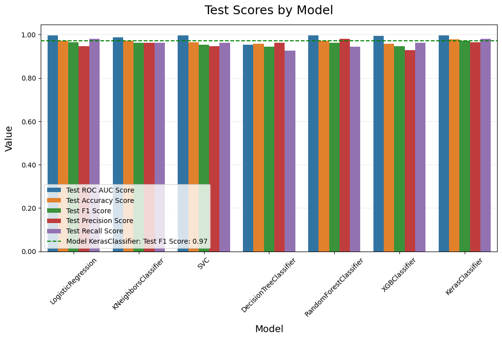
Compare Multi-Class Classification Models#
Let’s repeat the process, but with a multi-class dataset. Some of the binary classification metrics and charts disappear, but the comparison still works.
[145]:
# Create a sample multi-class classification dataset
X, y = load_iris(return_X_y=True)
X = pd.DataFrame(X, columns=['sepal_length', 'sepal_width', 'petal_length', 'petal_width'])
y = pd.Series(y)
class_map = {0: 'Setosa', 1: 'Versicolor', 2: 'Virginica'}
[146]:
# Set some variables referenced in the config
random_state = 42
class_weight = None
max_iter = 10000
# Set column lists referenced in the config
num_columns = list(X.columns)
cat_columns = []
# Define the callback for early stop, referenced by KerasClassifier
stopper = EarlyStopping(patience=4)
# Create a custom configuration file with model pipeline components and grid search params
my_config = {
'models' : {
'logreg': LogisticRegression(max_iter=max_iter, random_state=random_state, class_weight=class_weight),
'knn_class': KNeighborsClassifier(),
'svm_proba': SVC(random_state=random_state, probability=True, class_weight=class_weight),
'tree_class': DecisionTreeClassifier(random_state=random_state, class_weight=class_weight),
'forest_class': RandomForestClassifier(random_state=random_state, class_weight=class_weight),
'xgb_class': XGBClassifier(random_state=random_state),
'keras_class': KerasClassifier(model=dw.create_nn_multi, hidden_layer_dim=50, second_layer_dim=None,
third_layer_dim=None, dropout_rate=0.2, epochs=50, l2_reg=0.0,
verbose=0, class_weight=class_weight, random_state=random_state,
fit__validation_split=0.2, fit__callbacks=[stopper],
fit__batch_size=32, metrics=['accuracy'])
},
'scalers': {
'stand': StandardScaler(),
},
'params' : {
'logreg': {
'logreg__C': [0.0001, 0.001, 0.01, 0.1, 1, 10, 100],
'logreg__solver': ['newton-cg', 'lbfgs', 'saga']
},
'knn_class': {
'knn_class__n_neighbors': [3, 5, 10, 15, 20, 25],
'knn_class__weights': ['uniform', 'distance'],
'knn_class__metric': ['euclidean', 'manhattan']
},
'svm_proba': {
'svm_proba__C': [0.0001, 0.001, 0.01, 0.1, 1, 10, 100],
'svm_proba__kernel': ['linear', 'poly', 'rbf', 'sigmoid']
},
'tree_class': {
'tree_class__max_depth': [3, 5, 7],
'tree_class__min_samples_split': [5, 10, 15],
'tree_class__criterion': ['gini', 'entropy'],
'tree_class__min_samples_leaf': [2, 4, 6]
},
'forest_class': {
'forest_class__n_estimators' : [50, 100, 200],
'forest_class__max_depth': [3, 5, 7],
'forest_class__min_samples_split': [5, 10, 15],
'forest_class__criterion': ['gini', 'entropy'],
'forest_class__min_samples_leaf': [2, 4, 6]
},
'xgb_class': {
'xgb_class__learning_rate': [0.01, 0.1, 0.5],
'xgb_class__max_depth': [3, 5, 7],
'xgb_class__subsample': [0.7, 0.8, 0.9],
'xgb_class__colsample_bytree': [0.7, 0.8, 0.9],
'xgb_class__n_estimators': [50, 100, 200],
'xgb_class__objective': ['binary:logistic'],
'xgb_class__gamma': [0, 1, 5, 10]
},
'keras_class': {
'keras_class__loss': ['categorical_crossentropy'],
'keras_class__optimizer': ['adam'],
'keras_class__hidden_layer_dim': [50, 100, 200],
'keras_class__dropout_rate': [0.5],
'keras_class__l2_reg': [0.0],
'keras_class__second_layer_dim': [50, 100],
'keras_class__third_layer_dim': [None, 25, 50],
'keras_class__optimizer__learning_rate': [0.001],
'keras_class__fit__batch_size': [32]
}
},
'cv': {
'kfold_5': KFold(n_splits=5, shuffle=True, random_state=42),
},
'no_scale': ['tree_class', 'forest_class'],
'no_poly': ['knn_class', 'tree_class', 'forest_class', 'xgb_class']
}
[147]:
# Evaluate multiple classification models by searching for the best hyper-parameters and comparing results
multi_results_df = dw.compare_models(
# Data split and sampling
x=X, y=y, test_size=0.25, stratify=None, under_sample=None, over_sample=None, svm_knn_resample=None,
# Models and pipeline steps
imputer=None, transformers=None, scaler='stand', selector=None, svm_proba=True,
models=['logreg', 'knn_class', 'svm_proba', 'tree_class', 'forest_class', 'xgb_class', 'keras_class'],
# Grid search
search_type='random', scorer='accuracy', grid_cv='kfold_5', verbose=4,
# Model evaluation and charts
model_eval=True, plot_perf=True, plot_curve=True, fig_size=(12,6), legend_loc='lower left', rotation=45,
threshold=0.5, class_map=class_map, title='Iris',
# Config, preferences and notes
config=my_config, class_weight=None, random_state=42, decimal=4, n_jobs=None,
notes='X, Test Size=0.25, Standard Scaler, Random Grid (Accuracy), T=0.50'
)
-----------------------------------------------------------------------------------------
Starting Data Processing - May 30, 2024 09:22 AM UTC
-----------------------------------------------------------------------------------------
Classification type detected: multi
Unique values in y: [0 1 2]
Train/Test split, test_size: 0.25
X_train, X_test, y_train, y_test shapes: (112, 4) (38, 4) (112,) (38,)
-----------------------------------------------------------------------------------------
1/7: Starting LogisticRegression Random Search - May 30, 2024 09:22 AM UTC
-----------------------------------------------------------------------------------------
Fitting 5 folds for each of 10 candidates, totalling 50 fits
[CV 1/5] END logreg__C=0.0001, logreg__solver=newton-cg;, score=0.304 total time= 0.0s
[CV 2/5] END logreg__C=0.0001, logreg__solver=newton-cg;, score=0.261 total time= 0.0s
[CV 3/5] END logreg__C=0.0001, logreg__solver=newton-cg;, score=0.227 total time= 0.0s
[CV 4/5] END logreg__C=0.0001, logreg__solver=newton-cg;, score=0.273 total time= 0.0s
[CV 5/5] END logreg__C=0.0001, logreg__solver=newton-cg;, score=0.273 total time= 0.0s
[CV 1/5] END .logreg__C=10, logreg__solver=saga;, score=0.957 total time= 0.0s
[CV 2/5] END .logreg__C=10, logreg__solver=saga;, score=1.000 total time= 0.0s
[CV 3/5] END .logreg__C=10, logreg__solver=saga;, score=0.955 total time= 0.0s
[CV 4/5] END .logreg__C=10, logreg__solver=saga;, score=0.909 total time= 0.0s
[CV 5/5] END .logreg__C=10, logreg__solver=saga;, score=0.955 total time= 0.0s
[CV 1/5] END logreg__C=10, logreg__solver=newton-cg;, score=0.957 total time= 0.0s
[CV 2/5] END logreg__C=10, logreg__solver=newton-cg;, score=1.000 total time= 0.0s
[CV 3/5] END logreg__C=10, logreg__solver=newton-cg;, score=0.955 total time= 0.0s
[CV 4/5] END logreg__C=10, logreg__solver=newton-cg;, score=0.909 total time= 0.0s
[CV 5/5] END logreg__C=10, logreg__solver=newton-cg;, score=0.955 total time= 0.0s
[CV 1/5] END logreg__C=0.0001, logreg__solver=lbfgs;, score=0.304 total time= 0.0s
[CV 2/5] END logreg__C=0.0001, logreg__solver=lbfgs;, score=0.261 total time= 0.0s
[CV 3/5] END logreg__C=0.0001, logreg__solver=lbfgs;, score=0.227 total time= 0.0s
[CV 4/5] END logreg__C=0.0001, logreg__solver=lbfgs;, score=0.273 total time= 0.0s
[CV 5/5] END logreg__C=0.0001, logreg__solver=lbfgs;, score=0.273 total time= 0.0s
[CV 1/5] END logreg__C=0.01, logreg__solver=saga;, score=0.696 total time= 0.0s
[CV 2/5] END logreg__C=0.01, logreg__solver=saga;, score=0.913 total time= 0.0s
[CV 3/5] END logreg__C=0.01, logreg__solver=saga;, score=0.864 total time= 0.0s
[CV 4/5] END logreg__C=0.01, logreg__solver=saga;, score=0.818 total time= 0.0s
[CV 5/5] END logreg__C=0.01, logreg__solver=saga;, score=0.636 total time= 0.0s
[CV 1/5] END logreg__C=0.001, logreg__solver=saga;, score=0.522 total time= 0.0s
[CV 2/5] END logreg__C=0.001, logreg__solver=saga;, score=0.304 total time= 0.0s
[CV 3/5] END logreg__C=0.001, logreg__solver=saga;, score=0.273 total time= 0.0s
[CV 4/5] END logreg__C=0.001, logreg__solver=saga;, score=0.455 total time= 0.0s
[CV 5/5] END logreg__C=0.001, logreg__solver=saga;, score=0.500 total time= 0.0s
[CV 1/5] END logreg__C=0.1, logreg__solver=saga;, score=0.826 total time= 0.0s
[CV 2/5] END logreg__C=0.1, logreg__solver=saga;, score=1.000 total time= 0.0s
[CV 3/5] END logreg__C=0.1, logreg__solver=saga;, score=0.864 total time= 0.0s
[CV 4/5] END logreg__C=0.1, logreg__solver=saga;, score=0.818 total time= 0.0s
[CV 5/5] END logreg__C=0.1, logreg__solver=saga;, score=0.773 total time= 0.0s
[CV 1/5] END logreg__C=0.001, logreg__solver=newton-cg;, score=0.522 total time= 0.0s
[CV 2/5] END logreg__C=0.001, logreg__solver=newton-cg;, score=0.304 total time= 0.0s
[CV 3/5] END logreg__C=0.001, logreg__solver=newton-cg;, score=0.273 total time= 0.0s
[CV 4/5] END logreg__C=0.001, logreg__solver=newton-cg;, score=0.455 total time= 0.0s
[CV 5/5] END logreg__C=0.001, logreg__solver=newton-cg;, score=0.500 total time= 0.0s
[CV 1/5] END logreg__C=100, logreg__solver=newton-cg;, score=0.957 total time= 0.0s
[CV 2/5] END logreg__C=100, logreg__solver=newton-cg;, score=1.000 total time= 0.0s
[CV 3/5] END logreg__C=100, logreg__solver=newton-cg;, score=0.909 total time= 0.0s
[CV 4/5] END logreg__C=100, logreg__solver=newton-cg;, score=0.909 total time= 0.0s
[CV 5/5] END logreg__C=100, logreg__solver=newton-cg;, score=0.955 total time= 0.0s
[CV 1/5] END logreg__C=10, logreg__solver=lbfgs;, score=0.957 total time= 0.0s
[CV 2/5] END logreg__C=10, logreg__solver=lbfgs;, score=1.000 total time= 0.0s
[CV 3/5] END logreg__C=10, logreg__solver=lbfgs;, score=0.955 total time= 0.0s
[CV 4/5] END logreg__C=10, logreg__solver=lbfgs;, score=0.909 total time= 0.0s
[CV 5/5] END logreg__C=10, logreg__solver=lbfgs;, score=0.955 total time= 0.0s
Total Time: 0.3992 seconds
Average Fit Time: 0.0080 seconds
Inference Time: 0.0008
Best CV Accuracy Score: 0.9549
Train Accuracy Score: 0.9821
Test Accuracy Score: 1.0000
Overfit: No
Overfit Difference: -0.0179
Best Parameters: {'logreg__solver': 'saga', 'logreg__C': 10}
LogisticRegression Multi-Class Classification Report
precision recall f1-score support
Setosa 1.0000 1.0000 1.0000 15
Versicolor 1.0000 1.0000 1.0000 11
Virginica 1.0000 1.0000 1.0000 12
accuracy 1.0000 38
macro avg 1.0000 1.0000 1.0000 38
weighted avg 1.0000 1.0000 1.0000 38
ROC AUC: 1.0
Predicted Setosa Versicolor Virginica
Actual
Setosa 15 0 0
Versicolor 0 11 0
Virginica 0 0 12

-----------------------------------------------------------------------------------------
2/7: Starting KNeighborsClassifier Random Search - May 30, 2024 09:22 AM UTC
-----------------------------------------------------------------------------------------
Fitting 5 folds for each of 10 candidates, totalling 50 fits
[CV 1/5] END knn_class__metric=euclidean, knn_class__n_neighbors=20, knn_class__weights=uniform;, score=0.870 total time= 0.0s
[CV 2/5] END knn_class__metric=euclidean, knn_class__n_neighbors=20, knn_class__weights=uniform;, score=0.870 total time= 0.0s
[CV 3/5] END knn_class__metric=euclidean, knn_class__n_neighbors=20, knn_class__weights=uniform;, score=0.909 total time= 0.0s
[CV 4/5] END knn_class__metric=euclidean, knn_class__n_neighbors=20, knn_class__weights=uniform;, score=0.864 total time= 0.0s
[CV 5/5] END knn_class__metric=euclidean, knn_class__n_neighbors=20, knn_class__weights=uniform;, score=0.864 total time= 0.0s
[CV 1/5] END knn_class__metric=manhattan, knn_class__n_neighbors=10, knn_class__weights=uniform;, score=0.957 total time= 0.0s
[CV 2/5] END knn_class__metric=manhattan, knn_class__n_neighbors=10, knn_class__weights=uniform;, score=0.957 total time= 0.0s
[CV 3/5] END knn_class__metric=manhattan, knn_class__n_neighbors=10, knn_class__weights=uniform;, score=0.909 total time= 0.0s
[CV 4/5] END knn_class__metric=manhattan, knn_class__n_neighbors=10, knn_class__weights=uniform;, score=0.864 total time= 0.0s
[CV 5/5] END knn_class__metric=manhattan, knn_class__n_neighbors=10, knn_class__weights=uniform;, score=0.909 total time= 0.0s
[CV 1/5] END knn_class__metric=euclidean, knn_class__n_neighbors=3, knn_class__weights=uniform;, score=1.000 total time= 0.0s
[CV 2/5] END knn_class__metric=euclidean, knn_class__n_neighbors=3, knn_class__weights=uniform;, score=1.000 total time= 0.0s
[CV 3/5] END knn_class__metric=euclidean, knn_class__n_neighbors=3, knn_class__weights=uniform;, score=0.955 total time= 0.0s
[CV 4/5] END knn_class__metric=euclidean, knn_class__n_neighbors=3, knn_class__weights=uniform;, score=0.909 total time= 0.0s
[CV 5/5] END knn_class__metric=euclidean, knn_class__n_neighbors=3, knn_class__weights=uniform;, score=0.909 total time= 0.0s
[CV 1/5] END knn_class__metric=manhattan, knn_class__n_neighbors=15, knn_class__weights=uniform;, score=0.913 total time= 0.0s
[CV 2/5] END knn_class__metric=manhattan, knn_class__n_neighbors=15, knn_class__weights=uniform;, score=0.957 total time= 0.0s
[CV 3/5] END knn_class__metric=manhattan, knn_class__n_neighbors=15, knn_class__weights=uniform;, score=0.955 total time= 0.0s
[CV 4/5] END knn_class__metric=manhattan, knn_class__n_neighbors=15, knn_class__weights=uniform;, score=0.864 total time= 0.0s
[CV 5/5] END knn_class__metric=manhattan, knn_class__n_neighbors=15, knn_class__weights=uniform;, score=0.909 total time= 0.0s
[CV 1/5] END knn_class__metric=euclidean, knn_class__n_neighbors=25, knn_class__weights=distance;, score=0.913 total time= 0.0s
[CV 2/5] END knn_class__metric=euclidean, knn_class__n_neighbors=25, knn_class__weights=distance;, score=0.957 total time= 0.0s
[CV 3/5] END knn_class__metric=euclidean, knn_class__n_neighbors=25, knn_class__weights=distance;, score=0.909 total time= 0.0s
[CV 4/5] END knn_class__metric=euclidean, knn_class__n_neighbors=25, knn_class__weights=distance;, score=0.864 total time= 0.0s
[CV 5/5] END knn_class__metric=euclidean, knn_class__n_neighbors=25, knn_class__weights=distance;, score=0.909 total time= 0.0s
[CV 1/5] END knn_class__metric=euclidean, knn_class__n_neighbors=20, knn_class__weights=distance;, score=0.913 total time= 0.0s
[CV 2/5] END knn_class__metric=euclidean, knn_class__n_neighbors=20, knn_class__weights=distance;, score=1.000 total time= 0.0s
[CV 3/5] END knn_class__metric=euclidean, knn_class__n_neighbors=20, knn_class__weights=distance;, score=0.955 total time= 0.0s
[CV 4/5] END knn_class__metric=euclidean, knn_class__n_neighbors=20, knn_class__weights=distance;, score=0.864 total time= 0.0s
[CV 5/5] END knn_class__metric=euclidean, knn_class__n_neighbors=20, knn_class__weights=distance;, score=0.909 total time= 0.0s
[CV 1/5] END knn_class__metric=manhattan, knn_class__n_neighbors=3, knn_class__weights=distance;, score=0.913 total time= 0.0s
[CV 2/5] END knn_class__metric=manhattan, knn_class__n_neighbors=3, knn_class__weights=distance;, score=1.000 total time= 0.0s
[CV 3/5] END knn_class__metric=manhattan, knn_class__n_neighbors=3, knn_class__weights=distance;, score=0.955 total time= 0.0s
[CV 4/5] END knn_class__metric=manhattan, knn_class__n_neighbors=3, knn_class__weights=distance;, score=0.864 total time= 0.0s
[CV 5/5] END knn_class__metric=manhattan, knn_class__n_neighbors=3, knn_class__weights=distance;, score=0.909 total time= 0.0s
[CV 1/5] END knn_class__metric=euclidean, knn_class__n_neighbors=3, knn_class__weights=distance;, score=1.000 total time= 0.0s
[CV 2/5] END knn_class__metric=euclidean, knn_class__n_neighbors=3, knn_class__weights=distance;, score=1.000 total time= 0.0s
[CV 3/5] END knn_class__metric=euclidean, knn_class__n_neighbors=3, knn_class__weights=distance;, score=0.955 total time= 0.0s
[CV 4/5] END knn_class__metric=euclidean, knn_class__n_neighbors=3, knn_class__weights=distance;, score=0.909 total time= 0.0s
[CV 5/5] END knn_class__metric=euclidean, knn_class__n_neighbors=3, knn_class__weights=distance;, score=0.909 total time= 0.0s
[CV 1/5] END knn_class__metric=manhattan, knn_class__n_neighbors=20, knn_class__weights=distance;, score=0.913 total time= 0.0s
[CV 2/5] END knn_class__metric=manhattan, knn_class__n_neighbors=20, knn_class__weights=distance;, score=1.000 total time= 0.0s
[CV 3/5] END knn_class__metric=manhattan, knn_class__n_neighbors=20, knn_class__weights=distance;, score=0.909 total time= 0.0s
[CV 4/5] END knn_class__metric=manhattan, knn_class__n_neighbors=20, knn_class__weights=distance;, score=0.864 total time= 0.0s
[CV 5/5] END knn_class__metric=manhattan, knn_class__n_neighbors=20, knn_class__weights=distance;, score=0.909 total time= 0.0s
[CV 1/5] END knn_class__metric=euclidean, knn_class__n_neighbors=10, knn_class__weights=distance;, score=1.000 total time= 0.0s
[CV 2/5] END knn_class__metric=euclidean, knn_class__n_neighbors=10, knn_class__weights=distance;, score=1.000 total time= 0.0s
[CV 3/5] END knn_class__metric=euclidean, knn_class__n_neighbors=10, knn_class__weights=distance;, score=0.955 total time= 0.0s
[CV 4/5] END knn_class__metric=euclidean, knn_class__n_neighbors=10, knn_class__weights=distance;, score=0.864 total time= 0.0s
[CV 5/5] END knn_class__metric=euclidean, knn_class__n_neighbors=10, knn_class__weights=distance;, score=0.909 total time= 0.0s
Total Time: 0.3394 seconds
Average Fit Time: 0.0068 seconds
Inference Time: 0.0039
Best CV Accuracy Score: 0.9545
Train Accuracy Score: 0.9464
Test Accuracy Score: 1.0000
Overfit: No
Overfit Difference: -0.0536
Best Parameters: {'knn_class__weights': 'uniform', 'knn_class__n_neighbors': 3, 'knn_class__metric': 'euclidean'}
KNeighborsClassifier Multi-Class Classification Report
precision recall f1-score support
Setosa 1.0000 1.0000 1.0000 15
Versicolor 1.0000 1.0000 1.0000 11
Virginica 1.0000 1.0000 1.0000 12
accuracy 1.0000 38
macro avg 1.0000 1.0000 1.0000 38
weighted avg 1.0000 1.0000 1.0000 38
ROC AUC: 1.0
Predicted Setosa Versicolor Virginica
Actual
Setosa 15 0 0
Versicolor 0 11 0
Virginica 0 0 12

-----------------------------------------------------------------------------------------
3/7: Starting SVC Random Search - May 30, 2024 09:22 AM UTC
-----------------------------------------------------------------------------------------
Fitting 5 folds for each of 10 candidates, totalling 50 fits
[CV 1/5] END svm_proba__C=0.01, svm_proba__kernel=poly;, score=0.522 total time= 0.0s
[CV 2/5] END svm_proba__C=0.01, svm_proba__kernel=poly;, score=0.348 total time= 0.0s
[CV 3/5] END svm_proba__C=0.01, svm_proba__kernel=poly;, score=0.409 total time= 0.0s
[CV 4/5] END svm_proba__C=0.01, svm_proba__kernel=poly;, score=0.409 total time= 0.0s
[CV 5/5] END svm_proba__C=0.01, svm_proba__kernel=poly;, score=0.500 total time= 0.0s
[CV 1/5] END svm_proba__C=100, svm_proba__kernel=poly;, score=0.957 total time= 0.0s
[CV 2/5] END svm_proba__C=100, svm_proba__kernel=poly;, score=0.957 total time= 0.0s
[CV 3/5] END svm_proba__C=100, svm_proba__kernel=poly;, score=0.909 total time= 0.0s
[CV 4/5] END svm_proba__C=100, svm_proba__kernel=poly;, score=0.909 total time= 0.0s
[CV 5/5] END svm_proba__C=100, svm_proba__kernel=poly;, score=0.909 total time= 0.0s
[CV 1/5] END svm_proba__C=0.01, svm_proba__kernel=linear;, score=0.696 total time= 0.0s
[CV 2/5] END svm_proba__C=0.01, svm_proba__kernel=linear;, score=0.783 total time= 0.0s
[CV 3/5] END svm_proba__C=0.01, svm_proba__kernel=linear;, score=0.909 total time= 0.0s
[CV 4/5] END svm_proba__C=0.01, svm_proba__kernel=linear;, score=0.818 total time= 0.0s
[CV 5/5] END svm_proba__C=0.01, svm_proba__kernel=linear;, score=0.591 total time= 0.0s
[CV 1/5] END svm_proba__C=10, svm_proba__kernel=poly;, score=1.000 total time= 0.0s
[CV 2/5] END svm_proba__C=10, svm_proba__kernel=poly;, score=0.957 total time= 0.0s
[CV 3/5] END svm_proba__C=10, svm_proba__kernel=poly;, score=0.909 total time= 0.0s
[CV 4/5] END svm_proba__C=10, svm_proba__kernel=poly;, score=0.864 total time= 0.0s
[CV 5/5] END svm_proba__C=10, svm_proba__kernel=poly;, score=1.000 total time= 0.0s
[CV 1/5] END svm_proba__C=0.0001, svm_proba__kernel=linear;, score=0.304 total time= 0.0s
[CV 2/5] END svm_proba__C=0.0001, svm_proba__kernel=linear;, score=0.261 total time= 0.0s
[CV 3/5] END svm_proba__C=0.0001, svm_proba__kernel=linear;, score=0.227 total time= 0.0s
[CV 4/5] END svm_proba__C=0.0001, svm_proba__kernel=linear;, score=0.273 total time= 0.0s
[CV 5/5] END svm_proba__C=0.0001, svm_proba__kernel=linear;, score=0.273 total time= 0.0s
[CV 1/5] END svm_proba__C=0.1, svm_proba__kernel=linear;, score=0.957 total time= 0.0s
[CV 2/5] END svm_proba__C=0.1, svm_proba__kernel=linear;, score=1.000 total time= 0.0s
[CV 3/5] END svm_proba__C=0.1, svm_proba__kernel=linear;, score=0.909 total time= 0.0s
[CV 4/5] END svm_proba__C=0.1, svm_proba__kernel=linear;, score=0.909 total time= 0.0s
[CV 5/5] END svm_proba__C=0.1, svm_proba__kernel=linear;, score=0.909 total time= 0.0s
[CV 1/5] END svm_proba__C=1, svm_proba__kernel=poly;, score=0.913 total time= 0.0s
[CV 2/5] END svm_proba__C=1, svm_proba__kernel=poly;, score=0.826 total time= 0.0s
[CV 3/5] END svm_proba__C=1, svm_proba__kernel=poly;, score=0.818 total time= 0.0s
[CV 4/5] END svm_proba__C=1, svm_proba__kernel=poly;, score=0.909 total time= 0.0s
[CV 5/5] END svm_proba__C=1, svm_proba__kernel=poly;, score=1.000 total time= 0.0s
[CV 1/5] END svm_proba__C=10, svm_proba__kernel=rbf;, score=0.957 total time= 0.0s
[CV 2/5] END svm_proba__C=10, svm_proba__kernel=rbf;, score=1.000 total time= 0.0s
[CV 3/5] END svm_proba__C=10, svm_proba__kernel=rbf;, score=0.955 total time= 0.0s
[CV 4/5] END svm_proba__C=10, svm_proba__kernel=rbf;, score=0.909 total time= 0.0s
[CV 5/5] END svm_proba__C=10, svm_proba__kernel=rbf;, score=0.909 total time= 0.0s
[CV 1/5] END svm_proba__C=0.01, svm_proba__kernel=sigmoid;, score=0.304 total time= 0.0s
[CV 2/5] END svm_proba__C=0.01, svm_proba__kernel=sigmoid;, score=0.261 total time= 0.0s
[CV 3/5] END svm_proba__C=0.01, svm_proba__kernel=sigmoid;, score=0.227 total time= 0.0s
[CV 4/5] END svm_proba__C=0.01, svm_proba__kernel=sigmoid;, score=0.273 total time= 0.0s
[CV 5/5] END svm_proba__C=0.01, svm_proba__kernel=sigmoid;, score=0.273 total time= 0.0s
[CV 1/5] END svm_proba__C=0.1, svm_proba__kernel=poly;, score=0.870 total time= 0.0s
[CV 2/5] END svm_proba__C=0.1, svm_proba__kernel=poly;, score=0.783 total time= 0.0s
[CV 3/5] END svm_proba__C=0.1, svm_proba__kernel=poly;, score=0.773 total time= 0.0s
[CV 4/5] END svm_proba__C=0.1, svm_proba__kernel=poly;, score=0.727 total time= 0.0s
[CV 5/5] END svm_proba__C=0.1, svm_proba__kernel=poly;, score=0.909 total time= 0.0s
Total Time: 0.3629 seconds
Average Fit Time: 0.0073 seconds
Inference Time: 0.0012
Best CV Accuracy Score: 0.9458
Train Accuracy Score: 0.9821
Test Accuracy Score: 0.9737
Overfit: Yes
Overfit Difference: 0.0085
Best Parameters: {'svm_proba__kernel': 'rbf', 'svm_proba__C': 10}
SVC Multi-Class Classification Report
precision recall f1-score support
Setosa 1.0000 1.0000 1.0000 15
Versicolor 1.0000 0.9091 0.9524 11
Virginica 0.9231 1.0000 0.9600 12
accuracy 0.9737 38
macro avg 0.9744 0.9697 0.9708 38
weighted avg 0.9757 0.9737 0.9736 38
ROC AUC: 1.0
Predicted Setosa Versicolor Virginica
Actual
Setosa 15 0 0
Versicolor 0 10 1
Virginica 0 0 12
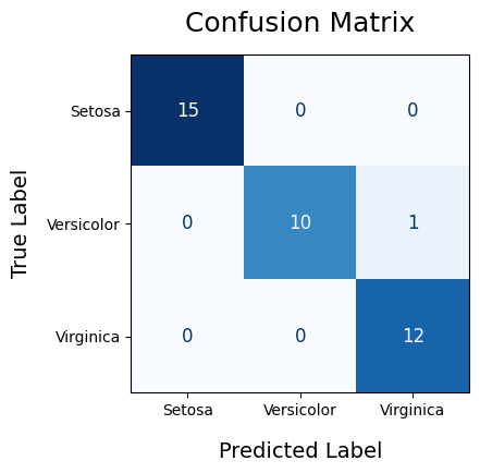
-----------------------------------------------------------------------------------------
4/7: Starting DecisionTreeClassifier Random Search - May 30, 2024 09:22 AM UTC
-----------------------------------------------------------------------------------------
Fitting 5 folds for each of 10 candidates, totalling 50 fits
[CV 1/5] END tree_class__criterion=gini, tree_class__max_depth=7, tree_class__min_samples_leaf=2, tree_class__min_samples_split=10;, score=0.870 total time= 0.0s
[CV 2/5] END tree_class__criterion=gini, tree_class__max_depth=7, tree_class__min_samples_leaf=2, tree_class__min_samples_split=10;, score=1.000 total time= 0.0s
[CV 3/5] END tree_class__criterion=gini, tree_class__max_depth=7, tree_class__min_samples_leaf=2, tree_class__min_samples_split=10;, score=0.909 total time= 0.0s
[CV 4/5] END tree_class__criterion=gini, tree_class__max_depth=7, tree_class__min_samples_leaf=2, tree_class__min_samples_split=10;, score=0.818 total time= 0.0s
[CV 5/5] END tree_class__criterion=gini, tree_class__max_depth=7, tree_class__min_samples_leaf=2, tree_class__min_samples_split=10;, score=0.909 total time= 0.0s
[CV 1/5] END tree_class__criterion=entropy, tree_class__max_depth=7, tree_class__min_samples_leaf=4, tree_class__min_samples_split=10;, score=0.913 total time= 0.0s
[CV 2/5] END tree_class__criterion=entropy, tree_class__max_depth=7, tree_class__min_samples_leaf=4, tree_class__min_samples_split=10;, score=0.913 total time= 0.0s
[CV 3/5] END tree_class__criterion=entropy, tree_class__max_depth=7, tree_class__min_samples_leaf=4, tree_class__min_samples_split=10;, score=1.000 total time= 0.0s
[CV 4/5] END tree_class__criterion=entropy, tree_class__max_depth=7, tree_class__min_samples_leaf=4, tree_class__min_samples_split=10;, score=0.818 total time= 0.0s
[CV 5/5] END tree_class__criterion=entropy, tree_class__max_depth=7, tree_class__min_samples_leaf=4, tree_class__min_samples_split=10;, score=0.909 total time= 0.0s
[CV 1/5] END tree_class__criterion=entropy, tree_class__max_depth=7, tree_class__min_samples_leaf=4, tree_class__min_samples_split=5;, score=1.000 total time= 0.0s
[CV 2/5] END tree_class__criterion=entropy, tree_class__max_depth=7, tree_class__min_samples_leaf=4, tree_class__min_samples_split=5;, score=0.957 total time= 0.0s
[CV 3/5] END tree_class__criterion=entropy, tree_class__max_depth=7, tree_class__min_samples_leaf=4, tree_class__min_samples_split=5;, score=1.000 total time= 0.0s
[CV 4/5] END tree_class__criterion=entropy, tree_class__max_depth=7, tree_class__min_samples_leaf=4, tree_class__min_samples_split=5;, score=0.818 total time= 0.0s
[CV 5/5] END tree_class__criterion=entropy, tree_class__max_depth=7, tree_class__min_samples_leaf=4, tree_class__min_samples_split=5;, score=0.909 total time= 0.0s
[CV 1/5] END tree_class__criterion=gini, tree_class__max_depth=5, tree_class__min_samples_leaf=4, tree_class__min_samples_split=5;, score=0.913 total time= 0.0s
[CV 2/5] END tree_class__criterion=gini, tree_class__max_depth=5, tree_class__min_samples_leaf=4, tree_class__min_samples_split=5;, score=1.000 total time= 0.0s
[CV 3/5] END tree_class__criterion=gini, tree_class__max_depth=5, tree_class__min_samples_leaf=4, tree_class__min_samples_split=5;, score=1.000 total time= 0.0s
[CV 4/5] END tree_class__criterion=gini, tree_class__max_depth=5, tree_class__min_samples_leaf=4, tree_class__min_samples_split=5;, score=0.818 total time= 0.0s
[CV 5/5] END tree_class__criterion=gini, tree_class__max_depth=5, tree_class__min_samples_leaf=4, tree_class__min_samples_split=5;, score=0.909 total time= 0.0s
[CV 1/5] END tree_class__criterion=entropy, tree_class__max_depth=5, tree_class__min_samples_leaf=6, tree_class__min_samples_split=15;, score=0.913 total time= 0.0s
[CV 2/5] END tree_class__criterion=entropy, tree_class__max_depth=5, tree_class__min_samples_leaf=6, tree_class__min_samples_split=15;, score=1.000 total time= 0.0s
[CV 3/5] END tree_class__criterion=entropy, tree_class__max_depth=5, tree_class__min_samples_leaf=6, tree_class__min_samples_split=15;, score=0.955 total time= 0.0s
[CV 4/5] END tree_class__criterion=entropy, tree_class__max_depth=5, tree_class__min_samples_leaf=6, tree_class__min_samples_split=15;, score=0.818 total time= 0.0s
[CV 5/5] END tree_class__criterion=entropy, tree_class__max_depth=5, tree_class__min_samples_leaf=6, tree_class__min_samples_split=15;, score=0.909 total time= 0.0s
[CV 1/5] END tree_class__criterion=gini, tree_class__max_depth=3, tree_class__min_samples_leaf=4, tree_class__min_samples_split=15;, score=0.913 total time= 0.0s
[CV 2/5] END tree_class__criterion=gini, tree_class__max_depth=3, tree_class__min_samples_leaf=4, tree_class__min_samples_split=15;, score=1.000 total time= 0.0s
[CV 3/5] END tree_class__criterion=gini, tree_class__max_depth=3, tree_class__min_samples_leaf=4, tree_class__min_samples_split=15;, score=1.000 total time= 0.0s
[CV 4/5] END tree_class__criterion=gini, tree_class__max_depth=3, tree_class__min_samples_leaf=4, tree_class__min_samples_split=15;, score=0.818 total time= 0.0s
[CV 5/5] END tree_class__criterion=gini, tree_class__max_depth=3, tree_class__min_samples_leaf=4, tree_class__min_samples_split=15;, score=0.909 total time= 0.0s
[CV 1/5] END tree_class__criterion=gini, tree_class__max_depth=5, tree_class__min_samples_leaf=6, tree_class__min_samples_split=15;, score=0.913 total time= 0.0s
[CV 2/5] END tree_class__criterion=gini, tree_class__max_depth=5, tree_class__min_samples_leaf=6, tree_class__min_samples_split=15;, score=1.000 total time= 0.0s
[CV 3/5] END tree_class__criterion=gini, tree_class__max_depth=5, tree_class__min_samples_leaf=6, tree_class__min_samples_split=15;, score=0.955 total time= 0.0s
[CV 4/5] END tree_class__criterion=gini, tree_class__max_depth=5, tree_class__min_samples_leaf=6, tree_class__min_samples_split=15;, score=0.818 total time= 0.0s
[CV 5/5] END tree_class__criterion=gini, tree_class__max_depth=5, tree_class__min_samples_leaf=6, tree_class__min_samples_split=15;, score=0.909 total time= 0.0s
[CV 1/5] END tree_class__criterion=entropy, tree_class__max_depth=7, tree_class__min_samples_leaf=6, tree_class__min_samples_split=10;, score=0.913 total time= 0.0s
[CV 2/5] END tree_class__criterion=entropy, tree_class__max_depth=7, tree_class__min_samples_leaf=6, tree_class__min_samples_split=10;, score=1.000 total time= 0.0s
[CV 3/5] END tree_class__criterion=entropy, tree_class__max_depth=7, tree_class__min_samples_leaf=6, tree_class__min_samples_split=10;, score=0.955 total time= 0.0s
[CV 4/5] END tree_class__criterion=entropy, tree_class__max_depth=7, tree_class__min_samples_leaf=6, tree_class__min_samples_split=10;, score=0.818 total time= 0.0s
[CV 5/5] END tree_class__criterion=entropy, tree_class__max_depth=7, tree_class__min_samples_leaf=6, tree_class__min_samples_split=10;, score=0.909 total time= 0.0s
[CV 1/5] END tree_class__criterion=gini, tree_class__max_depth=3, tree_class__min_samples_leaf=4, tree_class__min_samples_split=5;, score=0.913 total time= 0.0s
[CV 2/5] END tree_class__criterion=gini, tree_class__max_depth=3, tree_class__min_samples_leaf=4, tree_class__min_samples_split=5;, score=1.000 total time= 0.0s
[CV 3/5] END tree_class__criterion=gini, tree_class__max_depth=3, tree_class__min_samples_leaf=4, tree_class__min_samples_split=5;, score=1.000 total time= 0.0s
[CV 4/5] END tree_class__criterion=gini, tree_class__max_depth=3, tree_class__min_samples_leaf=4, tree_class__min_samples_split=5;, score=0.818 total time= 0.0s
[CV 5/5] END tree_class__criterion=gini, tree_class__max_depth=3, tree_class__min_samples_leaf=4, tree_class__min_samples_split=5;, score=0.909 total time= 0.0s
[CV 1/5] END tree_class__criterion=entropy, tree_class__max_depth=3, tree_class__min_samples_leaf=4, tree_class__min_samples_split=15;, score=0.913 total time= 0.1s
[CV 2/5] END tree_class__criterion=entropy, tree_class__max_depth=3, tree_class__min_samples_leaf=4, tree_class__min_samples_split=15;, score=1.000 total time= 0.0s
[CV 3/5] END tree_class__criterion=entropy, tree_class__max_depth=3, tree_class__min_samples_leaf=4, tree_class__min_samples_split=15;, score=1.000 total time= 0.0s
[CV 4/5] END tree_class__criterion=entropy, tree_class__max_depth=3, tree_class__min_samples_leaf=4, tree_class__min_samples_split=15;, score=0.818 total time= 0.0s
[CV 5/5] END tree_class__criterion=entropy, tree_class__max_depth=3, tree_class__min_samples_leaf=4, tree_class__min_samples_split=15;, score=0.909 total time= 0.0s
Total Time: 0.3191 seconds
Average Fit Time: 0.0064 seconds
Inference Time: 0.0009
Best CV Accuracy Score: 0.9368
Train Accuracy Score: 0.9643
Test Accuracy Score: 1.0000
Overfit: No
Overfit Difference: -0.0357
Best Parameters: {'tree_class__min_samples_split': 5, 'tree_class__min_samples_leaf': 4, 'tree_class__max_depth': 7, 'tree_class__criterion': 'entropy'}
DecisionTreeClassifier Multi-Class Classification Report
precision recall f1-score support
Setosa 1.0000 1.0000 1.0000 15
Versicolor 1.0000 1.0000 1.0000 11
Virginica 1.0000 1.0000 1.0000 12
accuracy 1.0000 38
macro avg 1.0000 1.0000 1.0000 38
weighted avg 1.0000 1.0000 1.0000 38
ROC AUC: 1.0
Predicted Setosa Versicolor Virginica
Actual
Setosa 15 0 0
Versicolor 0 11 0
Virginica 0 0 12
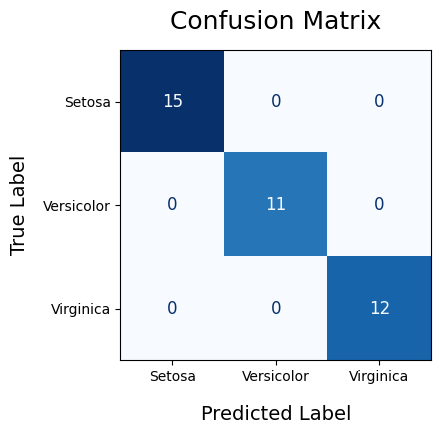
-----------------------------------------------------------------------------------------
5/7: Starting RandomForestClassifier Random Search - May 30, 2024 09:22 AM UTC
-----------------------------------------------------------------------------------------
Fitting 5 folds for each of 10 candidates, totalling 50 fits
[CV 1/5] END forest_class__criterion=entropy, forest_class__max_depth=7, forest_class__min_samples_leaf=6, forest_class__min_samples_split=10, forest_class__n_estimators=200;, score=0.913 total time= 0.2s
[CV 2/5] END forest_class__criterion=entropy, forest_class__max_depth=7, forest_class__min_samples_leaf=6, forest_class__min_samples_split=10, forest_class__n_estimators=200;, score=1.000 total time= 0.2s
[CV 3/5] END forest_class__criterion=entropy, forest_class__max_depth=7, forest_class__min_samples_leaf=6, forest_class__min_samples_split=10, forest_class__n_estimators=200;, score=0.955 total time= 0.3s
[CV 4/5] END forest_class__criterion=entropy, forest_class__max_depth=7, forest_class__min_samples_leaf=6, forest_class__min_samples_split=10, forest_class__n_estimators=200;, score=0.864 total time= 0.3s
[CV 5/5] END forest_class__criterion=entropy, forest_class__max_depth=7, forest_class__min_samples_leaf=6, forest_class__min_samples_split=10, forest_class__n_estimators=200;, score=0.909 total time= 0.3s
[CV 1/5] END forest_class__criterion=entropy, forest_class__max_depth=5, forest_class__min_samples_leaf=2, forest_class__min_samples_split=5, forest_class__n_estimators=100;, score=0.913 total time= 0.2s
[CV 2/5] END forest_class__criterion=entropy, forest_class__max_depth=5, forest_class__min_samples_leaf=2, forest_class__min_samples_split=5, forest_class__n_estimators=100;, score=1.000 total time= 0.1s
[CV 3/5] END forest_class__criterion=entropy, forest_class__max_depth=5, forest_class__min_samples_leaf=2, forest_class__min_samples_split=5, forest_class__n_estimators=100;, score=0.955 total time= 0.1s
[CV 4/5] END forest_class__criterion=entropy, forest_class__max_depth=5, forest_class__min_samples_leaf=2, forest_class__min_samples_split=5, forest_class__n_estimators=100;, score=0.864 total time= 0.1s
[CV 5/5] END forest_class__criterion=entropy, forest_class__max_depth=5, forest_class__min_samples_leaf=2, forest_class__min_samples_split=5, forest_class__n_estimators=100;, score=0.909 total time= 0.2s
[CV 1/5] END forest_class__criterion=entropy, forest_class__max_depth=5, forest_class__min_samples_leaf=6, forest_class__min_samples_split=10, forest_class__n_estimators=200;, score=0.913 total time= 0.3s
[CV 2/5] END forest_class__criterion=entropy, forest_class__max_depth=5, forest_class__min_samples_leaf=6, forest_class__min_samples_split=10, forest_class__n_estimators=200;, score=1.000 total time= 0.3s
[CV 3/5] END forest_class__criterion=entropy, forest_class__max_depth=5, forest_class__min_samples_leaf=6, forest_class__min_samples_split=10, forest_class__n_estimators=200;, score=0.955 total time= 0.2s
[CV 4/5] END forest_class__criterion=entropy, forest_class__max_depth=5, forest_class__min_samples_leaf=6, forest_class__min_samples_split=10, forest_class__n_estimators=200;, score=0.864 total time= 0.2s
[CV 5/5] END forest_class__criterion=entropy, forest_class__max_depth=5, forest_class__min_samples_leaf=6, forest_class__min_samples_split=10, forest_class__n_estimators=200;, score=0.909 total time= 0.2s
[CV 1/5] END forest_class__criterion=gini, forest_class__max_depth=7, forest_class__min_samples_leaf=2, forest_class__min_samples_split=5, forest_class__n_estimators=100;, score=0.913 total time= 0.1s
[CV 2/5] END forest_class__criterion=gini, forest_class__max_depth=7, forest_class__min_samples_leaf=2, forest_class__min_samples_split=5, forest_class__n_estimators=100;, score=1.000 total time= 0.2s
[CV 3/5] END forest_class__criterion=gini, forest_class__max_depth=7, forest_class__min_samples_leaf=2, forest_class__min_samples_split=5, forest_class__n_estimators=100;, score=0.955 total time= 0.1s
[CV 4/5] END forest_class__criterion=gini, forest_class__max_depth=7, forest_class__min_samples_leaf=2, forest_class__min_samples_split=5, forest_class__n_estimators=100;, score=0.864 total time= 0.1s
[CV 5/5] END forest_class__criterion=gini, forest_class__max_depth=7, forest_class__min_samples_leaf=2, forest_class__min_samples_split=5, forest_class__n_estimators=100;, score=0.909 total time= 0.1s
[CV 1/5] END forest_class__criterion=entropy, forest_class__max_depth=3, forest_class__min_samples_leaf=4, forest_class__min_samples_split=10, forest_class__n_estimators=100;, score=0.913 total time= 0.1s
[CV 2/5] END forest_class__criterion=entropy, forest_class__max_depth=3, forest_class__min_samples_leaf=4, forest_class__min_samples_split=10, forest_class__n_estimators=100;, score=1.000 total time= 0.1s
[CV 3/5] END forest_class__criterion=entropy, forest_class__max_depth=3, forest_class__min_samples_leaf=4, forest_class__min_samples_split=10, forest_class__n_estimators=100;, score=0.955 total time= 0.1s
[CV 4/5] END forest_class__criterion=entropy, forest_class__max_depth=3, forest_class__min_samples_leaf=4, forest_class__min_samples_split=10, forest_class__n_estimators=100;, score=0.864 total time= 0.1s
[CV 5/5] END forest_class__criterion=entropy, forest_class__max_depth=3, forest_class__min_samples_leaf=4, forest_class__min_samples_split=10, forest_class__n_estimators=100;, score=0.909 total time= 0.1s
[CV 1/5] END forest_class__criterion=gini, forest_class__max_depth=5, forest_class__min_samples_leaf=2, forest_class__min_samples_split=5, forest_class__n_estimators=200;, score=0.913 total time= 0.2s
[CV 2/5] END forest_class__criterion=gini, forest_class__max_depth=5, forest_class__min_samples_leaf=2, forest_class__min_samples_split=5, forest_class__n_estimators=200;, score=1.000 total time= 0.2s
[CV 3/5] END forest_class__criterion=gini, forest_class__max_depth=5, forest_class__min_samples_leaf=2, forest_class__min_samples_split=5, forest_class__n_estimators=200;, score=0.955 total time= 0.2s
[CV 4/5] END forest_class__criterion=gini, forest_class__max_depth=5, forest_class__min_samples_leaf=2, forest_class__min_samples_split=5, forest_class__n_estimators=200;, score=0.864 total time= 0.2s
[CV 5/5] END forest_class__criterion=gini, forest_class__max_depth=5, forest_class__min_samples_leaf=2, forest_class__min_samples_split=5, forest_class__n_estimators=200;, score=0.909 total time= 0.3s
[CV 1/5] END forest_class__criterion=entropy, forest_class__max_depth=3, forest_class__min_samples_leaf=6, forest_class__min_samples_split=5, forest_class__n_estimators=200;, score=0.913 total time= 0.3s
[CV 2/5] END forest_class__criterion=entropy, forest_class__max_depth=3, forest_class__min_samples_leaf=6, forest_class__min_samples_split=5, forest_class__n_estimators=200;, score=1.000 total time= 0.3s
[CV 3/5] END forest_class__criterion=entropy, forest_class__max_depth=3, forest_class__min_samples_leaf=6, forest_class__min_samples_split=5, forest_class__n_estimators=200;, score=0.955 total time= 0.3s
[CV 4/5] END forest_class__criterion=entropy, forest_class__max_depth=3, forest_class__min_samples_leaf=6, forest_class__min_samples_split=5, forest_class__n_estimators=200;, score=0.864 total time= 0.3s
[CV 5/5] END forest_class__criterion=entropy, forest_class__max_depth=3, forest_class__min_samples_leaf=6, forest_class__min_samples_split=5, forest_class__n_estimators=200;, score=0.909 total time= 0.3s
[CV 1/5] END forest_class__criterion=gini, forest_class__max_depth=5, forest_class__min_samples_leaf=6, forest_class__min_samples_split=15, forest_class__n_estimators=50;, score=0.913 total time= 0.1s
[CV 2/5] END forest_class__criterion=gini, forest_class__max_depth=5, forest_class__min_samples_leaf=6, forest_class__min_samples_split=15, forest_class__n_estimators=50;, score=1.000 total time= 0.1s
[CV 3/5] END forest_class__criterion=gini, forest_class__max_depth=5, forest_class__min_samples_leaf=6, forest_class__min_samples_split=15, forest_class__n_estimators=50;, score=1.000 total time= 0.1s
[CV 4/5] END forest_class__criterion=gini, forest_class__max_depth=5, forest_class__min_samples_leaf=6, forest_class__min_samples_split=15, forest_class__n_estimators=50;, score=0.864 total time= 0.1s
[CV 5/5] END forest_class__criterion=gini, forest_class__max_depth=5, forest_class__min_samples_leaf=6, forest_class__min_samples_split=15, forest_class__n_estimators=50;, score=0.909 total time= 0.1s
[CV 1/5] END forest_class__criterion=entropy, forest_class__max_depth=3, forest_class__min_samples_leaf=6, forest_class__min_samples_split=5, forest_class__n_estimators=100;, score=0.913 total time= 0.1s
[CV 2/5] END forest_class__criterion=entropy, forest_class__max_depth=3, forest_class__min_samples_leaf=6, forest_class__min_samples_split=5, forest_class__n_estimators=100;, score=1.000 total time= 0.2s
[CV 3/5] END forest_class__criterion=entropy, forest_class__max_depth=3, forest_class__min_samples_leaf=6, forest_class__min_samples_split=5, forest_class__n_estimators=100;, score=0.955 total time= 0.2s
[CV 4/5] END forest_class__criterion=entropy, forest_class__max_depth=3, forest_class__min_samples_leaf=6, forest_class__min_samples_split=5, forest_class__n_estimators=100;, score=0.864 total time= 0.2s
[CV 5/5] END forest_class__criterion=entropy, forest_class__max_depth=3, forest_class__min_samples_leaf=6, forest_class__min_samples_split=5, forest_class__n_estimators=100;, score=0.909 total time= 0.1s
[CV 1/5] END forest_class__criterion=entropy, forest_class__max_depth=7, forest_class__min_samples_leaf=4, forest_class__min_samples_split=5, forest_class__n_estimators=50;, score=0.913 total time= 0.1s
[CV 2/5] END forest_class__criterion=entropy, forest_class__max_depth=7, forest_class__min_samples_leaf=4, forest_class__min_samples_split=5, forest_class__n_estimators=50;, score=1.000 total time= 0.1s
[CV 3/5] END forest_class__criterion=entropy, forest_class__max_depth=7, forest_class__min_samples_leaf=4, forest_class__min_samples_split=5, forest_class__n_estimators=50;, score=0.955 total time= 0.1s
[CV 4/5] END forest_class__criterion=entropy, forest_class__max_depth=7, forest_class__min_samples_leaf=4, forest_class__min_samples_split=5, forest_class__n_estimators=50;, score=0.864 total time= 0.1s
[CV 5/5] END forest_class__criterion=entropy, forest_class__max_depth=7, forest_class__min_samples_leaf=4, forest_class__min_samples_split=5, forest_class__n_estimators=50;, score=0.909 total time= 0.1s
Total Time: 8.7033 seconds
Average Fit Time: 0.1741 seconds
Inference Time: 0.0031
Best CV Accuracy Score: 0.9372
Train Accuracy Score: 0.9643
Test Accuracy Score: 1.0000
Overfit: No
Overfit Difference: -0.0357
Best Parameters: {'forest_class__n_estimators': 50, 'forest_class__min_samples_split': 15, 'forest_class__min_samples_leaf': 6, 'forest_class__max_depth': 5, 'forest_class__criterion': 'gini'}
RandomForestClassifier Multi-Class Classification Report
precision recall f1-score support
Setosa 1.0000 1.0000 1.0000 15
Versicolor 1.0000 1.0000 1.0000 11
Virginica 1.0000 1.0000 1.0000 12
accuracy 1.0000 38
macro avg 1.0000 1.0000 1.0000 38
weighted avg 1.0000 1.0000 1.0000 38
ROC AUC: 1.0
Predicted Setosa Versicolor Virginica
Actual
Setosa 15 0 0
Versicolor 0 11 0
Virginica 0 0 12

-----------------------------------------------------------------------------------------
6/7: Starting XGBClassifier Random Search - May 30, 2024 09:22 AM UTC
-----------------------------------------------------------------------------------------
Fitting 5 folds for each of 10 candidates, totalling 50 fits
[CV 1/5] END xgb_class__colsample_bytree=0.9, xgb_class__gamma=1, xgb_class__learning_rate=0.1, xgb_class__max_depth=5, xgb_class__n_estimators=50, xgb_class__objective=binary:logistic, xgb_class__subsample=0.9;, score=0.913 total time= 0.2s
[CV 2/5] END xgb_class__colsample_bytree=0.9, xgb_class__gamma=1, xgb_class__learning_rate=0.1, xgb_class__max_depth=5, xgb_class__n_estimators=50, xgb_class__objective=binary:logistic, xgb_class__subsample=0.9;, score=1.000 total time= 0.3s
[CV 3/5] END xgb_class__colsample_bytree=0.9, xgb_class__gamma=1, xgb_class__learning_rate=0.1, xgb_class__max_depth=5, xgb_class__n_estimators=50, xgb_class__objective=binary:logistic, xgb_class__subsample=0.9;, score=0.955 total time= 0.1s
[CV 4/5] END xgb_class__colsample_bytree=0.9, xgb_class__gamma=1, xgb_class__learning_rate=0.1, xgb_class__max_depth=5, xgb_class__n_estimators=50, xgb_class__objective=binary:logistic, xgb_class__subsample=0.9;, score=0.864 total time= 0.2s
[CV 5/5] END xgb_class__colsample_bytree=0.9, xgb_class__gamma=1, xgb_class__learning_rate=0.1, xgb_class__max_depth=5, xgb_class__n_estimators=50, xgb_class__objective=binary:logistic, xgb_class__subsample=0.9;, score=0.864 total time= 0.2s
[CV 1/5] END xgb_class__colsample_bytree=0.7, xgb_class__gamma=0, xgb_class__learning_rate=0.5, xgb_class__max_depth=5, xgb_class__n_estimators=200, xgb_class__objective=binary:logistic, xgb_class__subsample=0.8;, score=0.870 total time= 0.7s
[CV 2/5] END xgb_class__colsample_bytree=0.7, xgb_class__gamma=0, xgb_class__learning_rate=0.5, xgb_class__max_depth=5, xgb_class__n_estimators=200, xgb_class__objective=binary:logistic, xgb_class__subsample=0.8;, score=0.957 total time= 0.7s
[CV 3/5] END xgb_class__colsample_bytree=0.7, xgb_class__gamma=0, xgb_class__learning_rate=0.5, xgb_class__max_depth=5, xgb_class__n_estimators=200, xgb_class__objective=binary:logistic, xgb_class__subsample=0.8;, score=0.955 total time= 0.6s
[CV 4/5] END xgb_class__colsample_bytree=0.7, xgb_class__gamma=0, xgb_class__learning_rate=0.5, xgb_class__max_depth=5, xgb_class__n_estimators=200, xgb_class__objective=binary:logistic, xgb_class__subsample=0.8;, score=0.864 total time= 0.4s
[CV 5/5] END xgb_class__colsample_bytree=0.7, xgb_class__gamma=0, xgb_class__learning_rate=0.5, xgb_class__max_depth=5, xgb_class__n_estimators=200, xgb_class__objective=binary:logistic, xgb_class__subsample=0.8;, score=0.864 total time= 0.5s
[CV 1/5] END xgb_class__colsample_bytree=0.9, xgb_class__gamma=5, xgb_class__learning_rate=0.1, xgb_class__max_depth=7, xgb_class__n_estimators=50, xgb_class__objective=binary:logistic, xgb_class__subsample=0.7;, score=0.913 total time= 0.1s
[CV 2/5] END xgb_class__colsample_bytree=0.9, xgb_class__gamma=5, xgb_class__learning_rate=0.1, xgb_class__max_depth=7, xgb_class__n_estimators=50, xgb_class__objective=binary:logistic, xgb_class__subsample=0.7;, score=1.000 total time= 0.1s
[CV 3/5] END xgb_class__colsample_bytree=0.9, xgb_class__gamma=5, xgb_class__learning_rate=0.1, xgb_class__max_depth=7, xgb_class__n_estimators=50, xgb_class__objective=binary:logistic, xgb_class__subsample=0.7;, score=0.955 total time= 0.1s
[CV 4/5] END xgb_class__colsample_bytree=0.9, xgb_class__gamma=5, xgb_class__learning_rate=0.1, xgb_class__max_depth=7, xgb_class__n_estimators=50, xgb_class__objective=binary:logistic, xgb_class__subsample=0.7;, score=0.864 total time= 0.1s
[CV 5/5] END xgb_class__colsample_bytree=0.9, xgb_class__gamma=5, xgb_class__learning_rate=0.1, xgb_class__max_depth=7, xgb_class__n_estimators=50, xgb_class__objective=binary:logistic, xgb_class__subsample=0.7;, score=0.864 total time= 0.1s
[CV 1/5] END xgb_class__colsample_bytree=0.8, xgb_class__gamma=1, xgb_class__learning_rate=0.5, xgb_class__max_depth=7, xgb_class__n_estimators=200, xgb_class__objective=binary:logistic, xgb_class__subsample=0.9;, score=0.957 total time= 0.4s
[CV 2/5] END xgb_class__colsample_bytree=0.8, xgb_class__gamma=1, xgb_class__learning_rate=0.5, xgb_class__max_depth=7, xgb_class__n_estimators=200, xgb_class__objective=binary:logistic, xgb_class__subsample=0.9;, score=1.000 total time= 0.4s
[CV 3/5] END xgb_class__colsample_bytree=0.8, xgb_class__gamma=1, xgb_class__learning_rate=0.5, xgb_class__max_depth=7, xgb_class__n_estimators=200, xgb_class__objective=binary:logistic, xgb_class__subsample=0.9;, score=0.955 total time= 0.4s
[CV 4/5] END xgb_class__colsample_bytree=0.8, xgb_class__gamma=1, xgb_class__learning_rate=0.5, xgb_class__max_depth=7, xgb_class__n_estimators=200, xgb_class__objective=binary:logistic, xgb_class__subsample=0.9;, score=0.864 total time= 0.5s
[CV 5/5] END xgb_class__colsample_bytree=0.8, xgb_class__gamma=1, xgb_class__learning_rate=0.5, xgb_class__max_depth=7, xgb_class__n_estimators=200, xgb_class__objective=binary:logistic, xgb_class__subsample=0.9;, score=0.864 total time= 0.4s
[CV 1/5] END xgb_class__colsample_bytree=0.8, xgb_class__gamma=10, xgb_class__learning_rate=0.5, xgb_class__max_depth=7, xgb_class__n_estimators=100, xgb_class__objective=binary:logistic, xgb_class__subsample=0.9;, score=0.913 total time= 0.2s
[CV 2/5] END xgb_class__colsample_bytree=0.8, xgb_class__gamma=10, xgb_class__learning_rate=0.5, xgb_class__max_depth=7, xgb_class__n_estimators=100, xgb_class__objective=binary:logistic, xgb_class__subsample=0.9;, score=1.000 total time= 0.2s
[CV 3/5] END xgb_class__colsample_bytree=0.8, xgb_class__gamma=10, xgb_class__learning_rate=0.5, xgb_class__max_depth=7, xgb_class__n_estimators=100, xgb_class__objective=binary:logistic, xgb_class__subsample=0.9;, score=0.955 total time= 0.2s
[CV 4/5] END xgb_class__colsample_bytree=0.8, xgb_class__gamma=10, xgb_class__learning_rate=0.5, xgb_class__max_depth=7, xgb_class__n_estimators=100, xgb_class__objective=binary:logistic, xgb_class__subsample=0.9;, score=0.864 total time= 0.1s
[CV 5/5] END xgb_class__colsample_bytree=0.8, xgb_class__gamma=10, xgb_class__learning_rate=0.5, xgb_class__max_depth=7, xgb_class__n_estimators=100, xgb_class__objective=binary:logistic, xgb_class__subsample=0.9;, score=0.864 total time= 0.2s
[CV 1/5] END xgb_class__colsample_bytree=0.8, xgb_class__gamma=5, xgb_class__learning_rate=0.1, xgb_class__max_depth=7, xgb_class__n_estimators=100, xgb_class__objective=binary:logistic, xgb_class__subsample=0.8;, score=0.913 total time= 0.2s
[CV 2/5] END xgb_class__colsample_bytree=0.8, xgb_class__gamma=5, xgb_class__learning_rate=0.1, xgb_class__max_depth=7, xgb_class__n_estimators=100, xgb_class__objective=binary:logistic, xgb_class__subsample=0.8;, score=1.000 total time= 0.2s
[CV 3/5] END xgb_class__colsample_bytree=0.8, xgb_class__gamma=5, xgb_class__learning_rate=0.1, xgb_class__max_depth=7, xgb_class__n_estimators=100, xgb_class__objective=binary:logistic, xgb_class__subsample=0.8;, score=0.955 total time= 0.2s
[CV 4/5] END xgb_class__colsample_bytree=0.8, xgb_class__gamma=5, xgb_class__learning_rate=0.1, xgb_class__max_depth=7, xgb_class__n_estimators=100, xgb_class__objective=binary:logistic, xgb_class__subsample=0.8;, score=0.864 total time= 0.2s
[CV 5/5] END xgb_class__colsample_bytree=0.8, xgb_class__gamma=5, xgb_class__learning_rate=0.1, xgb_class__max_depth=7, xgb_class__n_estimators=100, xgb_class__objective=binary:logistic, xgb_class__subsample=0.8;, score=0.864 total time= 0.2s
[CV 1/5] END xgb_class__colsample_bytree=0.7, xgb_class__gamma=10, xgb_class__learning_rate=0.1, xgb_class__max_depth=3, xgb_class__n_estimators=200, xgb_class__objective=binary:logistic, xgb_class__subsample=0.8;, score=0.913 total time= 0.5s
[CV 2/5] END xgb_class__colsample_bytree=0.7, xgb_class__gamma=10, xgb_class__learning_rate=0.1, xgb_class__max_depth=3, xgb_class__n_estimators=200, xgb_class__objective=binary:logistic, xgb_class__subsample=0.8;, score=1.000 total time= 0.5s
[CV 3/5] END xgb_class__colsample_bytree=0.7, xgb_class__gamma=10, xgb_class__learning_rate=0.1, xgb_class__max_depth=3, xgb_class__n_estimators=200, xgb_class__objective=binary:logistic, xgb_class__subsample=0.8;, score=0.955 total time= 0.8s
[CV 4/5] END xgb_class__colsample_bytree=0.7, xgb_class__gamma=10, xgb_class__learning_rate=0.1, xgb_class__max_depth=3, xgb_class__n_estimators=200, xgb_class__objective=binary:logistic, xgb_class__subsample=0.8;, score=0.864 total time= 1.0s
[CV 5/5] END xgb_class__colsample_bytree=0.7, xgb_class__gamma=10, xgb_class__learning_rate=0.1, xgb_class__max_depth=3, xgb_class__n_estimators=200, xgb_class__objective=binary:logistic, xgb_class__subsample=0.8;, score=0.864 total time= 0.6s
[CV 1/5] END xgb_class__colsample_bytree=0.7, xgb_class__gamma=10, xgb_class__learning_rate=0.1, xgb_class__max_depth=5, xgb_class__n_estimators=50, xgb_class__objective=binary:logistic, xgb_class__subsample=0.8;, score=0.913 total time= 0.1s
[CV 2/5] END xgb_class__colsample_bytree=0.7, xgb_class__gamma=10, xgb_class__learning_rate=0.1, xgb_class__max_depth=5, xgb_class__n_estimators=50, xgb_class__objective=binary:logistic, xgb_class__subsample=0.8;, score=1.000 total time= 0.1s
[CV 3/5] END xgb_class__colsample_bytree=0.7, xgb_class__gamma=10, xgb_class__learning_rate=0.1, xgb_class__max_depth=5, xgb_class__n_estimators=50, xgb_class__objective=binary:logistic, xgb_class__subsample=0.8;, score=1.000 total time= 0.1s
[CV 4/5] END xgb_class__colsample_bytree=0.7, xgb_class__gamma=10, xgb_class__learning_rate=0.1, xgb_class__max_depth=5, xgb_class__n_estimators=50, xgb_class__objective=binary:logistic, xgb_class__subsample=0.8;, score=0.864 total time= 0.1s
[CV 5/5] END xgb_class__colsample_bytree=0.7, xgb_class__gamma=10, xgb_class__learning_rate=0.1, xgb_class__max_depth=5, xgb_class__n_estimators=50, xgb_class__objective=binary:logistic, xgb_class__subsample=0.8;, score=0.864 total time= 0.1s
[CV 1/5] END xgb_class__colsample_bytree=0.9, xgb_class__gamma=10, xgb_class__learning_rate=0.5, xgb_class__max_depth=7, xgb_class__n_estimators=100, xgb_class__objective=binary:logistic, xgb_class__subsample=0.8;, score=0.913 total time= 0.3s
[CV 2/5] END xgb_class__colsample_bytree=0.9, xgb_class__gamma=10, xgb_class__learning_rate=0.5, xgb_class__max_depth=7, xgb_class__n_estimators=100, xgb_class__objective=binary:logistic, xgb_class__subsample=0.8;, score=1.000 total time= 0.2s
[CV 3/5] END xgb_class__colsample_bytree=0.9, xgb_class__gamma=10, xgb_class__learning_rate=0.5, xgb_class__max_depth=7, xgb_class__n_estimators=100, xgb_class__objective=binary:logistic, xgb_class__subsample=0.8;, score=0.955 total time= 0.2s
[CV 4/5] END xgb_class__colsample_bytree=0.9, xgb_class__gamma=10, xgb_class__learning_rate=0.5, xgb_class__max_depth=7, xgb_class__n_estimators=100, xgb_class__objective=binary:logistic, xgb_class__subsample=0.8;, score=0.864 total time= 0.2s
[CV 5/5] END xgb_class__colsample_bytree=0.9, xgb_class__gamma=10, xgb_class__learning_rate=0.5, xgb_class__max_depth=7, xgb_class__n_estimators=100, xgb_class__objective=binary:logistic, xgb_class__subsample=0.8;, score=0.864 total time= 0.2s
[CV 1/5] END xgb_class__colsample_bytree=0.9, xgb_class__gamma=5, xgb_class__learning_rate=0.5, xgb_class__max_depth=7, xgb_class__n_estimators=200, xgb_class__objective=binary:logistic, xgb_class__subsample=0.8;, score=0.870 total time= 0.3s
[CV 2/5] END xgb_class__colsample_bytree=0.9, xgb_class__gamma=5, xgb_class__learning_rate=0.5, xgb_class__max_depth=7, xgb_class__n_estimators=200, xgb_class__objective=binary:logistic, xgb_class__subsample=0.8;, score=1.000 total time= 0.4s
[CV 3/5] END xgb_class__colsample_bytree=0.9, xgb_class__gamma=5, xgb_class__learning_rate=0.5, xgb_class__max_depth=7, xgb_class__n_estimators=200, xgb_class__objective=binary:logistic, xgb_class__subsample=0.8;, score=1.000 total time= 0.3s
[CV 4/5] END xgb_class__colsample_bytree=0.9, xgb_class__gamma=5, xgb_class__learning_rate=0.5, xgb_class__max_depth=7, xgb_class__n_estimators=200, xgb_class__objective=binary:logistic, xgb_class__subsample=0.8;, score=0.864 total time= 0.3s
[CV 5/5] END xgb_class__colsample_bytree=0.9, xgb_class__gamma=5, xgb_class__learning_rate=0.5, xgb_class__max_depth=7, xgb_class__n_estimators=200, xgb_class__objective=binary:logistic, xgb_class__subsample=0.8;, score=0.864 total time= 0.4s
Total Time: 15.2190 seconds
Average Fit Time: 0.3044 seconds
Inference Time: 0.0024
Best CV Accuracy Score: 0.9281
Train Accuracy Score: 0.9643
Test Accuracy Score: 1.0000
Overfit: No
Overfit Difference: -0.0357
Best Parameters: {'xgb_class__subsample': 0.8, 'xgb_class__objective': 'binary:logistic', 'xgb_class__n_estimators': 50, 'xgb_class__max_depth': 5, 'xgb_class__learning_rate': 0.1, 'xgb_class__gamma': 10, 'xgb_class__colsample_bytree': 0.7}
XGBClassifier Multi-Class Classification Report
precision recall f1-score support
Setosa 1.0000 1.0000 1.0000 15
Versicolor 1.0000 1.0000 1.0000 11
Virginica 1.0000 1.0000 1.0000 12
accuracy 1.0000 38
macro avg 1.0000 1.0000 1.0000 38
weighted avg 1.0000 1.0000 1.0000 38
ROC AUC: 1.0
Predicted Setosa Versicolor Virginica
Actual
Setosa 15 0 0
Versicolor 0 11 0
Virginica 0 0 12

-----------------------------------------------------------------------------------------
7/7: Starting KerasClassifier Random Search - May 30, 2024 09:22 AM UTC
-----------------------------------------------------------------------------------------
Fitting 5 folds for each of 10 candidates, totalling 50 fits
[CV 1/5] END keras_class__dropout_rate=0.5, keras_class__fit__batch_size=32, keras_class__hidden_layer_dim=50, keras_class__l2_reg=0.0, keras_class__loss=categorical_crossentropy, keras_class__optimizer=adam, keras_class__optimizer__learning_rate=0.001, keras_class__second_layer_dim=50, keras_class__third_layer_dim=None;, score=0.696 total time= 3.3s
[CV 2/5] END keras_class__dropout_rate=0.5, keras_class__fit__batch_size=32, keras_class__hidden_layer_dim=50, keras_class__l2_reg=0.0, keras_class__loss=categorical_crossentropy, keras_class__optimizer=adam, keras_class__optimizer__learning_rate=0.001, keras_class__second_layer_dim=50, keras_class__third_layer_dim=None;, score=1.000 total time= 3.3s
[CV 3/5] END keras_class__dropout_rate=0.5, keras_class__fit__batch_size=32, keras_class__hidden_layer_dim=50, keras_class__l2_reg=0.0, keras_class__loss=categorical_crossentropy, keras_class__optimizer=adam, keras_class__optimizer__learning_rate=0.001, keras_class__second_layer_dim=50, keras_class__third_layer_dim=None;, score=0.909 total time= 3.6s
[CV 4/5] END keras_class__dropout_rate=0.5, keras_class__fit__batch_size=32, keras_class__hidden_layer_dim=50, keras_class__l2_reg=0.0, keras_class__loss=categorical_crossentropy, keras_class__optimizer=adam, keras_class__optimizer__learning_rate=0.001, keras_class__second_layer_dim=50, keras_class__third_layer_dim=None;, score=0.773 total time= 3.3s
[CV 5/5] END keras_class__dropout_rate=0.5, keras_class__fit__batch_size=32, keras_class__hidden_layer_dim=50, keras_class__l2_reg=0.0, keras_class__loss=categorical_crossentropy, keras_class__optimizer=adam, keras_class__optimizer__learning_rate=0.001, keras_class__second_layer_dim=50, keras_class__third_layer_dim=None;, score=0.682 total time= 3.2s
[CV 1/5] END keras_class__dropout_rate=0.5, keras_class__fit__batch_size=32, keras_class__hidden_layer_dim=50, keras_class__l2_reg=0.0, keras_class__loss=categorical_crossentropy, keras_class__optimizer=adam, keras_class__optimizer__learning_rate=0.001, keras_class__second_layer_dim=50, keras_class__third_layer_dim=25;, score=0.652 total time= 5.2s
[CV 2/5] END keras_class__dropout_rate=0.5, keras_class__fit__batch_size=32, keras_class__hidden_layer_dim=50, keras_class__l2_reg=0.0, keras_class__loss=categorical_crossentropy, keras_class__optimizer=adam, keras_class__optimizer__learning_rate=0.001, keras_class__second_layer_dim=50, keras_class__third_layer_dim=25;, score=1.000 total time= 9.1s
[CV 3/5] END keras_class__dropout_rate=0.5, keras_class__fit__batch_size=32, keras_class__hidden_layer_dim=50, keras_class__l2_reg=0.0, keras_class__loss=categorical_crossentropy, keras_class__optimizer=adam, keras_class__optimizer__learning_rate=0.001, keras_class__second_layer_dim=50, keras_class__third_layer_dim=25;, score=0.909 total time= 5.4s
[CV 4/5] END keras_class__dropout_rate=0.5, keras_class__fit__batch_size=32, keras_class__hidden_layer_dim=50, keras_class__l2_reg=0.0, keras_class__loss=categorical_crossentropy, keras_class__optimizer=adam, keras_class__optimizer__learning_rate=0.001, keras_class__second_layer_dim=50, keras_class__third_layer_dim=25;, score=0.773 total time= 4.0s
[CV 5/5] END keras_class__dropout_rate=0.5, keras_class__fit__batch_size=32, keras_class__hidden_layer_dim=50, keras_class__l2_reg=0.0, keras_class__loss=categorical_crossentropy, keras_class__optimizer=adam, keras_class__optimizer__learning_rate=0.001, keras_class__second_layer_dim=50, keras_class__third_layer_dim=25;, score=0.682 total time= 4.1s
[CV 1/5] END keras_class__dropout_rate=0.5, keras_class__fit__batch_size=32, keras_class__hidden_layer_dim=100, keras_class__l2_reg=0.0, keras_class__loss=categorical_crossentropy, keras_class__optimizer=adam, keras_class__optimizer__learning_rate=0.001, keras_class__second_layer_dim=50, keras_class__third_layer_dim=50;, score=0.739 total time= 3.8s
[CV 2/5] END keras_class__dropout_rate=0.5, keras_class__fit__batch_size=32, keras_class__hidden_layer_dim=100, keras_class__l2_reg=0.0, keras_class__loss=categorical_crossentropy, keras_class__optimizer=adam, keras_class__optimizer__learning_rate=0.001, keras_class__second_layer_dim=50, keras_class__third_layer_dim=50;, score=1.000 total time= 3.8s
[CV 3/5] END keras_class__dropout_rate=0.5, keras_class__fit__batch_size=32, keras_class__hidden_layer_dim=100, keras_class__l2_reg=0.0, keras_class__loss=categorical_crossentropy, keras_class__optimizer=adam, keras_class__optimizer__learning_rate=0.001, keras_class__second_layer_dim=50, keras_class__third_layer_dim=50;, score=0.909 total time= 3.7s
[CV 4/5] END keras_class__dropout_rate=0.5, keras_class__fit__batch_size=32, keras_class__hidden_layer_dim=100, keras_class__l2_reg=0.0, keras_class__loss=categorical_crossentropy, keras_class__optimizer=adam, keras_class__optimizer__learning_rate=0.001, keras_class__second_layer_dim=50, keras_class__third_layer_dim=50;, score=0.773 total time= 4.4s
[CV 5/5] END keras_class__dropout_rate=0.5, keras_class__fit__batch_size=32, keras_class__hidden_layer_dim=100, keras_class__l2_reg=0.0, keras_class__loss=categorical_crossentropy, keras_class__optimizer=adam, keras_class__optimizer__learning_rate=0.001, keras_class__second_layer_dim=50, keras_class__third_layer_dim=50;, score=0.773 total time= 3.9s
[CV 1/5] END keras_class__dropout_rate=0.5, keras_class__fit__batch_size=32, keras_class__hidden_layer_dim=50, keras_class__l2_reg=0.0, keras_class__loss=categorical_crossentropy, keras_class__optimizer=adam, keras_class__optimizer__learning_rate=0.001, keras_class__second_layer_dim=100, keras_class__third_layer_dim=50;, score=0.696 total time= 4.6s
[CV 2/5] END keras_class__dropout_rate=0.5, keras_class__fit__batch_size=32, keras_class__hidden_layer_dim=50, keras_class__l2_reg=0.0, keras_class__loss=categorical_crossentropy, keras_class__optimizer=adam, keras_class__optimizer__learning_rate=0.001, keras_class__second_layer_dim=100, keras_class__third_layer_dim=50;, score=1.000 total time= 4.7s
[CV 3/5] END keras_class__dropout_rate=0.5, keras_class__fit__batch_size=32, keras_class__hidden_layer_dim=50, keras_class__l2_reg=0.0, keras_class__loss=categorical_crossentropy, keras_class__optimizer=adam, keras_class__optimizer__learning_rate=0.001, keras_class__second_layer_dim=100, keras_class__third_layer_dim=50;, score=0.909 total time= 5.1s
[CV 4/5] END keras_class__dropout_rate=0.5, keras_class__fit__batch_size=32, keras_class__hidden_layer_dim=50, keras_class__l2_reg=0.0, keras_class__loss=categorical_crossentropy, keras_class__optimizer=adam, keras_class__optimizer__learning_rate=0.001, keras_class__second_layer_dim=100, keras_class__third_layer_dim=50;, score=0.773 total time= 4.6s
[CV 5/5] END keras_class__dropout_rate=0.5, keras_class__fit__batch_size=32, keras_class__hidden_layer_dim=50, keras_class__l2_reg=0.0, keras_class__loss=categorical_crossentropy, keras_class__optimizer=adam, keras_class__optimizer__learning_rate=0.001, keras_class__second_layer_dim=100, keras_class__third_layer_dim=50;, score=0.682 total time= 3.9s
[CV 1/5] END keras_class__dropout_rate=0.5, keras_class__fit__batch_size=32, keras_class__hidden_layer_dim=50, keras_class__l2_reg=0.0, keras_class__loss=categorical_crossentropy, keras_class__optimizer=adam, keras_class__optimizer__learning_rate=0.001, keras_class__second_layer_dim=100, keras_class__third_layer_dim=None;, score=0.739 total time= 3.4s
[CV 2/5] END keras_class__dropout_rate=0.5, keras_class__fit__batch_size=32, keras_class__hidden_layer_dim=50, keras_class__l2_reg=0.0, keras_class__loss=categorical_crossentropy, keras_class__optimizer=adam, keras_class__optimizer__learning_rate=0.001, keras_class__second_layer_dim=100, keras_class__third_layer_dim=None;, score=1.000 total time= 4.0s
[CV 3/5] END keras_class__dropout_rate=0.5, keras_class__fit__batch_size=32, keras_class__hidden_layer_dim=50, keras_class__l2_reg=0.0, keras_class__loss=categorical_crossentropy, keras_class__optimizer=adam, keras_class__optimizer__learning_rate=0.001, keras_class__second_layer_dim=100, keras_class__third_layer_dim=None;, score=0.864 total time= 3.3s
[CV 4/5] END keras_class__dropout_rate=0.5, keras_class__fit__batch_size=32, keras_class__hidden_layer_dim=50, keras_class__l2_reg=0.0, keras_class__loss=categorical_crossentropy, keras_class__optimizer=adam, keras_class__optimizer__learning_rate=0.001, keras_class__second_layer_dim=100, keras_class__third_layer_dim=None;, score=0.773 total time= 3.3s
[CV 5/5] END keras_class__dropout_rate=0.5, keras_class__fit__batch_size=32, keras_class__hidden_layer_dim=50, keras_class__l2_reg=0.0, keras_class__loss=categorical_crossentropy, keras_class__optimizer=adam, keras_class__optimizer__learning_rate=0.001, keras_class__second_layer_dim=100, keras_class__third_layer_dim=None;, score=0.682 total time= 3.4s
[CV 1/5] END keras_class__dropout_rate=0.5, keras_class__fit__batch_size=32, keras_class__hidden_layer_dim=200, keras_class__l2_reg=0.0, keras_class__loss=categorical_crossentropy, keras_class__optimizer=adam, keras_class__optimizer__learning_rate=0.001, keras_class__second_layer_dim=50, keras_class__third_layer_dim=25;, score=0.739 total time= 4.4s
[CV 2/5] END keras_class__dropout_rate=0.5, keras_class__fit__batch_size=32, keras_class__hidden_layer_dim=200, keras_class__l2_reg=0.0, keras_class__loss=categorical_crossentropy, keras_class__optimizer=adam, keras_class__optimizer__learning_rate=0.001, keras_class__second_layer_dim=50, keras_class__third_layer_dim=25;, score=1.000 total time= 4.4s
[CV 3/5] END keras_class__dropout_rate=0.5, keras_class__fit__batch_size=32, keras_class__hidden_layer_dim=200, keras_class__l2_reg=0.0, keras_class__loss=categorical_crossentropy, keras_class__optimizer=adam, keras_class__optimizer__learning_rate=0.001, keras_class__second_layer_dim=50, keras_class__third_layer_dim=25;, score=0.864 total time= 3.9s
[CV 4/5] END keras_class__dropout_rate=0.5, keras_class__fit__batch_size=32, keras_class__hidden_layer_dim=200, keras_class__l2_reg=0.0, keras_class__loss=categorical_crossentropy, keras_class__optimizer=adam, keras_class__optimizer__learning_rate=0.001, keras_class__second_layer_dim=50, keras_class__third_layer_dim=25;, score=0.773 total time= 4.2s
[CV 5/5] END keras_class__dropout_rate=0.5, keras_class__fit__batch_size=32, keras_class__hidden_layer_dim=200, keras_class__l2_reg=0.0, keras_class__loss=categorical_crossentropy, keras_class__optimizer=adam, keras_class__optimizer__learning_rate=0.001, keras_class__second_layer_dim=50, keras_class__third_layer_dim=25;, score=0.682 total time= 4.1s
[CV 1/5] END keras_class__dropout_rate=0.5, keras_class__fit__batch_size=32, keras_class__hidden_layer_dim=200, keras_class__l2_reg=0.0, keras_class__loss=categorical_crossentropy, keras_class__optimizer=adam, keras_class__optimizer__learning_rate=0.001, keras_class__second_layer_dim=100, keras_class__third_layer_dim=25;, score=0.739 total time= 3.9s
[CV 2/5] END keras_class__dropout_rate=0.5, keras_class__fit__batch_size=32, keras_class__hidden_layer_dim=200, keras_class__l2_reg=0.0, keras_class__loss=categorical_crossentropy, keras_class__optimizer=adam, keras_class__optimizer__learning_rate=0.001, keras_class__second_layer_dim=100, keras_class__third_layer_dim=25;, score=1.000 total time= 3.9s
[CV 3/5] END keras_class__dropout_rate=0.5, keras_class__fit__batch_size=32, keras_class__hidden_layer_dim=200, keras_class__l2_reg=0.0, keras_class__loss=categorical_crossentropy, keras_class__optimizer=adam, keras_class__optimizer__learning_rate=0.001, keras_class__second_layer_dim=100, keras_class__third_layer_dim=25;, score=0.909 total time= 3.8s
[CV 4/5] END keras_class__dropout_rate=0.5, keras_class__fit__batch_size=32, keras_class__hidden_layer_dim=200, keras_class__l2_reg=0.0, keras_class__loss=categorical_crossentropy, keras_class__optimizer=adam, keras_class__optimizer__learning_rate=0.001, keras_class__second_layer_dim=100, keras_class__third_layer_dim=25;, score=0.773 total time= 3.7s
[CV 5/5] END keras_class__dropout_rate=0.5, keras_class__fit__batch_size=32, keras_class__hidden_layer_dim=200, keras_class__l2_reg=0.0, keras_class__loss=categorical_crossentropy, keras_class__optimizer=adam, keras_class__optimizer__learning_rate=0.001, keras_class__second_layer_dim=100, keras_class__third_layer_dim=25;, score=0.773 total time= 3.8s
[CV 1/5] END keras_class__dropout_rate=0.5, keras_class__fit__batch_size=32, keras_class__hidden_layer_dim=200, keras_class__l2_reg=0.0, keras_class__loss=categorical_crossentropy, keras_class__optimizer=adam, keras_class__optimizer__learning_rate=0.001, keras_class__second_layer_dim=100, keras_class__third_layer_dim=None;, score=0.739 total time= 3.2s
[CV 2/5] END keras_class__dropout_rate=0.5, keras_class__fit__batch_size=32, keras_class__hidden_layer_dim=200, keras_class__l2_reg=0.0, keras_class__loss=categorical_crossentropy, keras_class__optimizer=adam, keras_class__optimizer__learning_rate=0.001, keras_class__second_layer_dim=100, keras_class__third_layer_dim=None;, score=1.000 total time= 4.2s
[CV 3/5] END keras_class__dropout_rate=0.5, keras_class__fit__batch_size=32, keras_class__hidden_layer_dim=200, keras_class__l2_reg=0.0, keras_class__loss=categorical_crossentropy, keras_class__optimizer=adam, keras_class__optimizer__learning_rate=0.001, keras_class__second_layer_dim=100, keras_class__third_layer_dim=None;, score=0.909 total time= 3.4s
[CV 4/5] END keras_class__dropout_rate=0.5, keras_class__fit__batch_size=32, keras_class__hidden_layer_dim=200, keras_class__l2_reg=0.0, keras_class__loss=categorical_crossentropy, keras_class__optimizer=adam, keras_class__optimizer__learning_rate=0.001, keras_class__second_layer_dim=100, keras_class__third_layer_dim=None;, score=0.818 total time= 4.3s
[CV 5/5] END keras_class__dropout_rate=0.5, keras_class__fit__batch_size=32, keras_class__hidden_layer_dim=200, keras_class__l2_reg=0.0, keras_class__loss=categorical_crossentropy, keras_class__optimizer=adam, keras_class__optimizer__learning_rate=0.001, keras_class__second_layer_dim=100, keras_class__third_layer_dim=None;, score=0.818 total time= 4.2s
[CV 1/5] END keras_class__dropout_rate=0.5, keras_class__fit__batch_size=32, keras_class__hidden_layer_dim=100, keras_class__l2_reg=0.0, keras_class__loss=categorical_crossentropy, keras_class__optimizer=adam, keras_class__optimizer__learning_rate=0.001, keras_class__second_layer_dim=100, keras_class__third_layer_dim=50;, score=0.739 total time= 3.8s
[CV 2/5] END keras_class__dropout_rate=0.5, keras_class__fit__batch_size=32, keras_class__hidden_layer_dim=100, keras_class__l2_reg=0.0, keras_class__loss=categorical_crossentropy, keras_class__optimizer=adam, keras_class__optimizer__learning_rate=0.001, keras_class__second_layer_dim=100, keras_class__third_layer_dim=50;, score=1.000 total time= 4.0s
[CV 3/5] END keras_class__dropout_rate=0.5, keras_class__fit__batch_size=32, keras_class__hidden_layer_dim=100, keras_class__l2_reg=0.0, keras_class__loss=categorical_crossentropy, keras_class__optimizer=adam, keras_class__optimizer__learning_rate=0.001, keras_class__second_layer_dim=100, keras_class__third_layer_dim=50;, score=0.864 total time= 3.9s
[CV 4/5] END keras_class__dropout_rate=0.5, keras_class__fit__batch_size=32, keras_class__hidden_layer_dim=100, keras_class__l2_reg=0.0, keras_class__loss=categorical_crossentropy, keras_class__optimizer=adam, keras_class__optimizer__learning_rate=0.001, keras_class__second_layer_dim=100, keras_class__third_layer_dim=50;, score=0.773 total time= 3.4s
[CV 5/5] END keras_class__dropout_rate=0.5, keras_class__fit__batch_size=32, keras_class__hidden_layer_dim=100, keras_class__l2_reg=0.0, keras_class__loss=categorical_crossentropy, keras_class__optimizer=adam, keras_class__optimizer__learning_rate=0.001, keras_class__second_layer_dim=100, keras_class__third_layer_dim=50;, score=0.682 total time= 4.3s
[CV 1/5] END keras_class__dropout_rate=0.5, keras_class__fit__batch_size=32, keras_class__hidden_layer_dim=50, keras_class__l2_reg=0.0, keras_class__loss=categorical_crossentropy, keras_class__optimizer=adam, keras_class__optimizer__learning_rate=0.001, keras_class__second_layer_dim=50, keras_class__third_layer_dim=50;, score=0.696 total time= 3.7s
[CV 2/5] END keras_class__dropout_rate=0.5, keras_class__fit__batch_size=32, keras_class__hidden_layer_dim=50, keras_class__l2_reg=0.0, keras_class__loss=categorical_crossentropy, keras_class__optimizer=adam, keras_class__optimizer__learning_rate=0.001, keras_class__second_layer_dim=50, keras_class__third_layer_dim=50;, score=1.000 total time= 3.4s
[CV 3/5] END keras_class__dropout_rate=0.5, keras_class__fit__batch_size=32, keras_class__hidden_layer_dim=50, keras_class__l2_reg=0.0, keras_class__loss=categorical_crossentropy, keras_class__optimizer=adam, keras_class__optimizer__learning_rate=0.001, keras_class__second_layer_dim=50, keras_class__third_layer_dim=50;, score=0.909 total time= 3.4s
[CV 4/5] END keras_class__dropout_rate=0.5, keras_class__fit__batch_size=32, keras_class__hidden_layer_dim=50, keras_class__l2_reg=0.0, keras_class__loss=categorical_crossentropy, keras_class__optimizer=adam, keras_class__optimizer__learning_rate=0.001, keras_class__second_layer_dim=50, keras_class__third_layer_dim=50;, score=0.773 total time= 3.7s
[CV 5/5] END keras_class__dropout_rate=0.5, keras_class__fit__batch_size=32, keras_class__hidden_layer_dim=50, keras_class__l2_reg=0.0, keras_class__loss=categorical_crossentropy, keras_class__optimizer=adam, keras_class__optimizer__learning_rate=0.001, keras_class__second_layer_dim=50, keras_class__third_layer_dim=50;, score=0.682 total time= 13.4s
Total Time: 216.1515 seconds
Average Fit Time: 4.3230 seconds
Inference Time: 0.0748
Best CV Accuracy Score: 0.8569
Train Accuracy Score: 0.9554
Test Accuracy Score: 1.0000
Overfit: No
Overfit Difference: -0.0446
Best Parameters: {'keras_class__third_layer_dim': None, 'keras_class__second_layer_dim': 100, 'keras_class__optimizer__learning_rate': 0.001, 'keras_class__optimizer': 'adam', 'keras_class__loss': 'categorical_crossentropy', 'keras_class__l2_reg': 0.0, 'keras_class__hidden_layer_dim': 200, 'keras_class__fit__batch_size': 32, 'keras_class__dropout_rate': 0.5}
Model: "Sequential"
┏━━━━━━━━━━━━━━━━━━━━━━━━━━━━━━━━━┳━━━━━━━━━━━━━━━━━━━━━━━━┳━━━━━━━━━━━━━━━┓ ┃ Layer (type) ┃ Output Shape ┃ Param # ┃ ┡━━━━━━━━━━━━━━━━━━━━━━━━━━━━━━━━━╇━━━━━━━━━━━━━━━━━━━━━━━━╇━━━━━━━━━━━━━━━┩ │ Hidden_1 (Dense) │ (None, 200) │ 1,000 │ ├─────────────────────────────────┼────────────────────────┼───────────────┤ │ Dropout_1 (Dropout) │ (None, 200) │ 0 │ ├─────────────────────────────────┼────────────────────────┼───────────────┤ │ Hidden_2 (Dense) │ (None, 100) │ 20,100 │ ├─────────────────────────────────┼────────────────────────┼───────────────┤ │ Dropout_2 (Dropout) │ (None, 100) │ 0 │ ├─────────────────────────────────┼────────────────────────┼───────────────┤ │ Output (Dense) │ (None, 3) │ 303 │ └─────────────────────────────────┴────────────────────────┴───────────────┘
Total params: 64,211 (250.83 KB)
Trainable params: 21,403 (83.61 KB)
Non-trainable params: 0 (0.00 B)
Optimizer params: 42,808 (167.22 KB)
KerasClassifier Multi-Class Classification Report
precision recall f1-score support
Setosa 1.0000 1.0000 1.0000 15
Versicolor 1.0000 1.0000 1.0000 11
Virginica 1.0000 1.0000 1.0000 12
accuracy 1.0000 38
macro avg 1.0000 1.0000 1.0000 38
weighted avg 1.0000 1.0000 1.0000 38
ROC AUC: 1.0
Predicted Setosa Versicolor Virginica
Actual
Setosa 15 0 0
Versicolor 0 11 0
Virginica 0 0 12

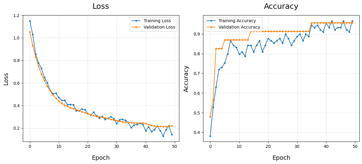
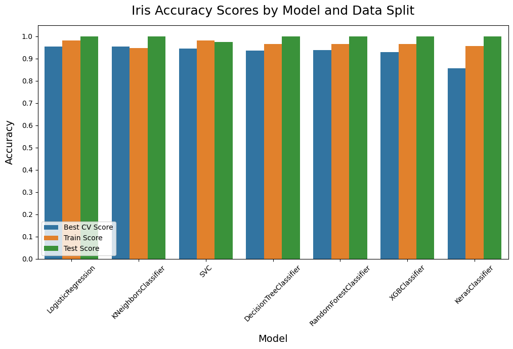
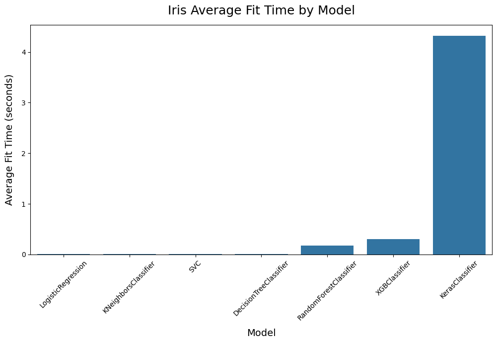
Create Binary Classification Neural Network#
dw.create_nn_binary() creates a binary classification neural network model.
This function allows for flexible configuration of the neural network structure for binary classification using the KerasClassifier in scikit-learn. It supports adding up to three hidden layers with customizable dimensions, dropout regularization, and L2 regularization.
Use this function to create a neural network model with a specific structure and regularization settings for binary classification tasks. It is set as the model parameter of a KerasClassifier instance referenced in the configuration file for dw.compare_models.
[148]:
# Create a sample classification dataset
X, y = make_classification(n_samples=1000, n_features=10, random_state=42)
X_train, X_test, y_train, y_test = train_test_split(X, y, test_size=0.2, random_state=42)
# Define the metadata that would be passed from KerasClassifier
meta = {"n_features_in_": 10, "X_shape_": (80, 10)}
[149]:
# Create a basic neural network with default settings
model = dw.create_nn_binary(hidden_layer_dim=32, dropout_rate=0.2, l2_reg=0.01, meta=meta)
# Review the model summary
model.summary()
Model: "Sequential"
┏━━━━━━━━━━━━━━━━━━━━━━━━━━━━━━━━━┳━━━━━━━━━━━━━━━━━━━━━━━━┳━━━━━━━━━━━━━━━┓ ┃ Layer (type) ┃ Output Shape ┃ Param # ┃ ┡━━━━━━━━━━━━━━━━━━━━━━━━━━━━━━━━━╇━━━━━━━━━━━━━━━━━━━━━━━━╇━━━━━━━━━━━━━━━┩ │ Hidden_1 (Dense) │ (None, 32) │ 352 │ ├─────────────────────────────────┼────────────────────────┼───────────────┤ │ Dropout_1 (Dropout) │ (None, 32) │ 0 │ ├─────────────────────────────────┼────────────────────────┼───────────────┤ │ Output (Dense) │ (None, 1) │ 33 │ └─────────────────────────────────┴────────────────────────┴───────────────┘
Total params: 385 (1.50 KB)
Trainable params: 385 (1.50 KB)
Non-trainable params: 0 (0.00 B)
[150]:
# Create a neural network with additional layers and regularization
model = dw.create_nn_binary(hidden_layer_dim=64, dropout_rate=0.3, l2_reg=0.05,
second_layer_dim=32, third_layer_dim=16, meta=meta)
# Review the model summary
model.summary()
Model: "Sequential"
┏━━━━━━━━━━━━━━━━━━━━━━━━━━━━━━━━━┳━━━━━━━━━━━━━━━━━━━━━━━━┳━━━━━━━━━━━━━━━┓ ┃ Layer (type) ┃ Output Shape ┃ Param # ┃ ┡━━━━━━━━━━━━━━━━━━━━━━━━━━━━━━━━━╇━━━━━━━━━━━━━━━━━━━━━━━━╇━━━━━━━━━━━━━━━┩ │ Hidden_1 (Dense) │ (None, 64) │ 704 │ ├─────────────────────────────────┼────────────────────────┼───────────────┤ │ Dropout_1 (Dropout) │ (None, 64) │ 0 │ ├─────────────────────────────────┼────────────────────────┼───────────────┤ │ Hidden_2 (Dense) │ (None, 32) │ 2,080 │ ├─────────────────────────────────┼────────────────────────┼───────────────┤ │ Dropout_2 (Dropout) │ (None, 32) │ 0 │ ├─────────────────────────────────┼────────────────────────┼───────────────┤ │ Hidden_3 (Dense) │ (None, 16) │ 528 │ ├─────────────────────────────────┼────────────────────────┼───────────────┤ │ Dropout_3 (Dropout) │ (None, 16) │ 0 │ ├─────────────────────────────────┼────────────────────────┼───────────────┤ │ Output (Dense) │ (None, 1) │ 17 │ └─────────────────────────────────┴────────────────────────┴───────────────┘
Total params: 3,329 (13.00 KB)
Trainable params: 3,329 (13.00 KB)
Non-trainable params: 0 (0.00 B)
[151]:
# Compile the model
model.compile(optimizer='Adam', loss='binary_crossentropy', metrics=['accuracy'])
[152]:
# Fit the model
model.fit(X_train, y_train, epochs=50, validation_split=0.2, shuffle=True)
Epoch 1/50
20/20 ━━━━━━━━━━━━━━━━━━━━ 2s 12ms/step - accuracy: 0.5465 - loss: 4.5624 - val_accuracy: 0.7437 - val_loss: 4.0054
Epoch 2/50
20/20 ━━━━━━━━━━━━━━━━━━━━ 0s 3ms/step - accuracy: 0.5945 - loss: 3.8493 - val_accuracy: 0.7750 - val_loss: 3.3740
Epoch 3/50
20/20 ━━━━━━━━━━━━━━━━━━━━ 0s 4ms/step - accuracy: 0.7194 - loss: 3.2314 - val_accuracy: 0.8375 - val_loss: 2.8437
Epoch 4/50
20/20 ━━━━━━━━━━━━━━━━━━━━ 0s 3ms/step - accuracy: 0.7780 - loss: 2.7182 - val_accuracy: 0.8375 - val_loss: 2.3995
Epoch 5/50
20/20 ━━━━━━━━━━━━━━━━━━━━ 0s 4ms/step - accuracy: 0.8188 - loss: 2.2949 - val_accuracy: 0.8562 - val_loss: 2.0287
Epoch 6/50
20/20 ━━━━━━━━━━━━━━━━━━━━ 0s 3ms/step - accuracy: 0.8514 - loss: 1.9501 - val_accuracy: 0.8687 - val_loss: 1.7202
Epoch 7/50
20/20 ━━━━━━━━━━━━━━━━━━━━ 0s 8ms/step - accuracy: 0.8587 - loss: 1.6467 - val_accuracy: 0.8750 - val_loss: 1.4680
Epoch 8/50
20/20 ━━━━━━━━━━━━━━━━━━━━ 0s 3ms/step - accuracy: 0.8490 - loss: 1.4198 - val_accuracy: 0.8750 - val_loss: 1.2664
Epoch 9/50
20/20 ━━━━━━━━━━━━━━━━━━━━ 0s 3ms/step - accuracy: 0.8605 - loss: 1.2370 - val_accuracy: 0.8750 - val_loss: 1.1052
Epoch 10/50
20/20 ━━━━━━━━━━━━━━━━━━━━ 0s 3ms/step - accuracy: 0.8466 - loss: 1.0839 - val_accuracy: 0.8687 - val_loss: 0.9770
Epoch 11/50
20/20 ━━━━━━━━━━━━━━━━━━━━ 0s 3ms/step - accuracy: 0.8831 - loss: 0.9437 - val_accuracy: 0.8687 - val_loss: 0.8743
Epoch 12/50
20/20 ━━━━━━━━━━━━━━━━━━━━ 0s 4ms/step - accuracy: 0.8659 - loss: 0.8623 - val_accuracy: 0.8687 - val_loss: 0.7932
Epoch 13/50
20/20 ━━━━━━━━━━━━━━━━━━━━ 0s 3ms/step - accuracy: 0.8576 - loss: 0.7798 - val_accuracy: 0.8687 - val_loss: 0.7295
Epoch 14/50
20/20 ━━━━━━━━━━━━━━━━━━━━ 0s 3ms/step - accuracy: 0.8361 - loss: 0.7316 - val_accuracy: 0.8687 - val_loss: 0.6779
Epoch 15/50
20/20 ━━━━━━━━━━━━━━━━━━━━ 0s 3ms/step - accuracy: 0.8564 - loss: 0.6754 - val_accuracy: 0.8625 - val_loss: 0.6366
Epoch 16/50
20/20 ━━━━━━━━━━━━━━━━━━━━ 0s 3ms/step - accuracy: 0.8695 - loss: 0.6150 - val_accuracy: 0.8625 - val_loss: 0.6063
Epoch 17/50
20/20 ━━━━━━━━━━━━━━━━━━━━ 0s 4ms/step - accuracy: 0.8625 - loss: 0.6024 - val_accuracy: 0.8625 - val_loss: 0.5803
Epoch 18/50
20/20 ━━━━━━━━━━━━━━━━━━━━ 0s 8ms/step - accuracy: 0.8704 - loss: 0.5755 - val_accuracy: 0.8625 - val_loss: 0.5608
Epoch 19/50
20/20 ━━━━━━━━━━━━━━━━━━━━ 0s 3ms/step - accuracy: 0.8712 - loss: 0.5585 - val_accuracy: 0.8562 - val_loss: 0.5449
Epoch 20/50
20/20 ━━━━━━━━━━━━━━━━━━━━ 0s 3ms/step - accuracy: 0.8796 - loss: 0.5350 - val_accuracy: 0.8625 - val_loss: 0.5359
Epoch 21/50
20/20 ━━━━━━━━━━━━━━━━━━━━ 0s 4ms/step - accuracy: 0.8756 - loss: 0.5094 - val_accuracy: 0.8625 - val_loss: 0.5269
Epoch 22/50
20/20 ━━━━━━━━━━━━━━━━━━━━ 0s 3ms/step - accuracy: 0.8470 - loss: 0.5304 - val_accuracy: 0.8625 - val_loss: 0.5156
Epoch 23/50
20/20 ━━━━━━━━━━━━━━━━━━━━ 0s 3ms/step - accuracy: 0.8638 - loss: 0.5149 - val_accuracy: 0.8625 - val_loss: 0.5073
Epoch 24/50
20/20 ━━━━━━━━━━━━━━━━━━━━ 0s 3ms/step - accuracy: 0.8637 - loss: 0.5026 - val_accuracy: 0.8562 - val_loss: 0.5044
Epoch 25/50
20/20 ━━━━━━━━━━━━━━━━━━━━ 0s 3ms/step - accuracy: 0.8711 - loss: 0.4832 - val_accuracy: 0.8562 - val_loss: 0.5002
Epoch 26/50
20/20 ━━━━━━━━━━━━━━━━━━━━ 0s 3ms/step - accuracy: 0.8642 - loss: 0.4935 - val_accuracy: 0.8625 - val_loss: 0.4966
Epoch 27/50
20/20 ━━━━━━━━━━━━━━━━━━━━ 0s 3ms/step - accuracy: 0.8662 - loss: 0.4689 - val_accuracy: 0.8625 - val_loss: 0.4971
Epoch 28/50
20/20 ━━━━━━━━━━━━━━━━━━━━ 0s 3ms/step - accuracy: 0.8748 - loss: 0.4767 - val_accuracy: 0.8625 - val_loss: 0.4897
Epoch 29/50
20/20 ━━━━━━━━━━━━━━━━━━━━ 0s 3ms/step - accuracy: 0.8765 - loss: 0.4768 - val_accuracy: 0.8562 - val_loss: 0.4856
Epoch 30/50
20/20 ━━━━━━━━━━━━━━━━━━━━ 0s 2ms/step - accuracy: 0.8666 - loss: 0.4752 - val_accuracy: 0.8625 - val_loss: 0.4869
Epoch 31/50
20/20 ━━━━━━━━━━━━━━━━━━━━ 0s 2ms/step - accuracy: 0.8726 - loss: 0.4772 - val_accuracy: 0.8625 - val_loss: 0.4884
Epoch 32/50
20/20 ━━━━━━━━━━━━━━━━━━━━ 0s 2ms/step - accuracy: 0.8725 - loss: 0.4773 - val_accuracy: 0.8562 - val_loss: 0.4843
Epoch 33/50
20/20 ━━━━━━━━━━━━━━━━━━━━ 0s 3ms/step - accuracy: 0.8578 - loss: 0.4773 - val_accuracy: 0.8625 - val_loss: 0.4907
Epoch 34/50
20/20 ━━━━━━━━━━━━━━━━━━━━ 0s 3ms/step - accuracy: 0.8504 - loss: 0.4856 - val_accuracy: 0.8562 - val_loss: 0.4816
Epoch 35/50
20/20 ━━━━━━━━━━━━━━━━━━━━ 0s 3ms/step - accuracy: 0.8752 - loss: 0.4727 - val_accuracy: 0.8625 - val_loss: 0.4815
Epoch 36/50
20/20 ━━━━━━━━━━━━━━━━━━━━ 0s 3ms/step - accuracy: 0.8635 - loss: 0.4765 - val_accuracy: 0.8562 - val_loss: 0.4823
Epoch 37/50
20/20 ━━━━━━━━━━━━━━━━━━━━ 0s 3ms/step - accuracy: 0.8791 - loss: 0.4622 - val_accuracy: 0.8562 - val_loss: 0.4809
Epoch 38/50
20/20 ━━━━━━━━━━━━━━━━━━━━ 0s 4ms/step - accuracy: 0.8749 - loss: 0.4788 - val_accuracy: 0.8562 - val_loss: 0.4776
Epoch 39/50
20/20 ━━━━━━━━━━━━━━━━━━━━ 0s 3ms/step - accuracy: 0.8453 - loss: 0.4720 - val_accuracy: 0.8562 - val_loss: 0.4757
Epoch 40/50
20/20 ━━━━━━━━━━━━━━━━━━━━ 0s 3ms/step - accuracy: 0.8564 - loss: 0.4694 - val_accuracy: 0.8625 - val_loss: 0.4734
Epoch 41/50
20/20 ━━━━━━━━━━━━━━━━━━━━ 0s 3ms/step - accuracy: 0.8626 - loss: 0.4800 - val_accuracy: 0.8687 - val_loss: 0.4738
Epoch 42/50
20/20 ━━━━━━━━━━━━━━━━━━━━ 0s 3ms/step - accuracy: 0.8579 - loss: 0.4614 - val_accuracy: 0.8687 - val_loss: 0.4705
Epoch 43/50
20/20 ━━━━━━━━━━━━━━━━━━━━ 0s 4ms/step - accuracy: 0.8517 - loss: 0.4719 - val_accuracy: 0.8687 - val_loss: 0.4742
Epoch 44/50
20/20 ━━━━━━━━━━━━━━━━━━━━ 0s 3ms/step - accuracy: 0.8601 - loss: 0.4575 - val_accuracy: 0.8687 - val_loss: 0.4764
Epoch 45/50
20/20 ━━━━━━━━━━━━━━━━━━━━ 0s 3ms/step - accuracy: 0.8484 - loss: 0.4763 - val_accuracy: 0.8625 - val_loss: 0.4745
Epoch 46/50
20/20 ━━━━━━━━━━━━━━━━━━━━ 0s 3ms/step - accuracy: 0.8657 - loss: 0.4630 - val_accuracy: 0.8562 - val_loss: 0.4699
Epoch 47/50
20/20 ━━━━━━━━━━━━━━━━━━━━ 0s 4ms/step - accuracy: 0.8525 - loss: 0.4570 - val_accuracy: 0.8625 - val_loss: 0.4722
Epoch 48/50
20/20 ━━━━━━━━━━━━━━━━━━━━ 0s 3ms/step - accuracy: 0.8631 - loss: 0.4676 - val_accuracy: 0.8625 - val_loss: 0.4718
Epoch 49/50
20/20 ━━━━━━━━━━━━━━━━━━━━ 0s 4ms/step - accuracy: 0.8789 - loss: 0.4570 - val_accuracy: 0.8687 - val_loss: 0.4716
Epoch 50/50
20/20 ━━━━━━━━━━━━━━━━━━━━ 0s 4ms/step - accuracy: 0.8806 - loss: 0.4489 - val_accuracy: 0.8687 - val_loss: 0.4724
[152]:
<keras.src.callbacks.history.History at 0x7fe839f96f10>
[153]:
# Plot the training history, including loss and accuracy
dw.plot_train_history(model)
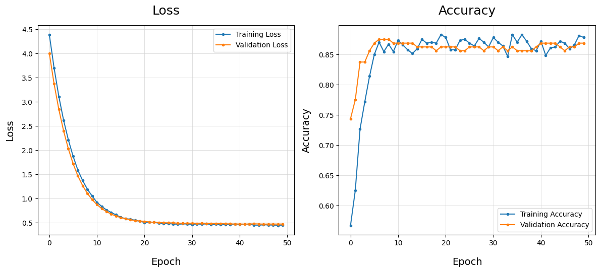
Create Multi-Class Classification Neural Network#
dw.create_nn_multi() creates a multi-class classification neural network model.
This function allows for flexible configuration of the neural network structure for multi-class classification using the KerasClassifier in scikit-learn. It supports adding an optional hidden layer with customizable dimensions, dropout regularization, and L2 regularization.
Use this function to create a neural network model with a specific structure and regularization settings for multi-class classification tasks. It is set as the model parameter of a KerasClassifier instance referenced in the configuration file for dw.compare_models.
[154]:
# Create a sample classification dataset
X, y = load_iris(return_X_y=True)
X_train, X_test, y_train, y_test = train_test_split(X, y, test_size=0.2, random_state=42)
# Define the metadata that would be passed from KerasClassifier
meta = {"n_features_in_": 4, "X_shape_": (120, 4), "n_classes_": 3}
[155]:
# One-hot encode labels
y_train = to_categorical(y_train, num_classes=3)
y_test = to_categorical(y_test, num_classes=3)
[156]:
# Create a basic neural network with default settings:
model = dw.create_nn_multi(hidden_layer_dim=64, dropout_rate=0.2, l2_reg=0.01, meta=meta)
# Review the model summary
model.summary()
Model: "Sequential"
┏━━━━━━━━━━━━━━━━━━━━━━━━━━━━━━━━━┳━━━━━━━━━━━━━━━━━━━━━━━━┳━━━━━━━━━━━━━━━┓ ┃ Layer (type) ┃ Output Shape ┃ Param # ┃ ┡━━━━━━━━━━━━━━━━━━━━━━━━━━━━━━━━━╇━━━━━━━━━━━━━━━━━━━━━━━━╇━━━━━━━━━━━━━━━┩ │ Hidden_1 (Dense) │ (None, 64) │ 320 │ ├─────────────────────────────────┼────────────────────────┼───────────────┤ │ Dropout_1 (Dropout) │ (None, 64) │ 0 │ ├─────────────────────────────────┼────────────────────────┼───────────────┤ │ Output (Dense) │ (None, 3) │ 195 │ └─────────────────────────────────┴────────────────────────┴───────────────┘
Total params: 515 (2.01 KB)
Trainable params: 515 (2.01 KB)
Non-trainable params: 0 (0.00 B)
[157]:
# Create a neural network with an additional hidden layer
model = dw.create_nn_multi(hidden_layer_dim=128, dropout_rate=0.3, l2_reg=0.05,
second_layer_dim=64, meta=meta)
# Review the model summary
model.summary()
Model: "Sequential"
┏━━━━━━━━━━━━━━━━━━━━━━━━━━━━━━━━━┳━━━━━━━━━━━━━━━━━━━━━━━━┳━━━━━━━━━━━━━━━┓ ┃ Layer (type) ┃ Output Shape ┃ Param # ┃ ┡━━━━━━━━━━━━━━━━━━━━━━━━━━━━━━━━━╇━━━━━━━━━━━━━━━━━━━━━━━━╇━━━━━━━━━━━━━━━┩ │ Hidden_1 (Dense) │ (None, 128) │ 640 │ ├─────────────────────────────────┼────────────────────────┼───────────────┤ │ Dropout_1 (Dropout) │ (None, 128) │ 0 │ ├─────────────────────────────────┼────────────────────────┼───────────────┤ │ Hidden_2 (Dense) │ (None, 64) │ 8,256 │ ├─────────────────────────────────┼────────────────────────┼───────────────┤ │ Dropout_2 (Dropout) │ (None, 64) │ 0 │ ├─────────────────────────────────┼────────────────────────┼───────────────┤ │ Output (Dense) │ (None, 3) │ 195 │ └─────────────────────────────────┴────────────────────────┴───────────────┘
Total params: 9,091 (35.51 KB)
Trainable params: 9,091 (35.51 KB)
Non-trainable params: 0 (0.00 B)
[158]:
# Compile the model
model.compile(optimizer='Adam', loss='categorical_crossentropy', metrics=['accuracy'])
[159]:
# Fit the model
model.fit(X_train, y_train, epochs=50, validation_split=0.2, shuffle=True)
Epoch 1/50
3/3 ━━━━━━━━━━━━━━━━━━━━ 1s 123ms/step - accuracy: 0.3268 - loss: 5.9623 - val_accuracy: 0.2500 - val_loss: 5.6886
Epoch 2/50
3/3 ━━━━━━━━━━━━━━━━━━━━ 0s 13ms/step - accuracy: 0.3359 - loss: 5.6368 - val_accuracy: 0.5000 - val_loss: 5.4026
Epoch 3/50
3/3 ━━━━━━━━━━━━━━━━━━━━ 0s 13ms/step - accuracy: 0.4349 - loss: 5.3491 - val_accuracy: 0.5000 - val_loss: 5.1600
Epoch 4/50
3/3 ━━━━━━━━━━━━━━━━━━━━ 0s 17ms/step - accuracy: 0.4401 - loss: 5.1631 - val_accuracy: 0.5000 - val_loss: 4.9341
Epoch 5/50
3/3 ━━━━━━━━━━━━━━━━━━━━ 0s 15ms/step - accuracy: 0.4271 - loss: 4.9947 - val_accuracy: 0.5000 - val_loss: 4.7216
Epoch 6/50
3/3 ━━━━━━━━━━━━━━━━━━━━ 0s 18ms/step - accuracy: 0.5078 - loss: 4.7129 - val_accuracy: 0.5417 - val_loss: 4.5287
Epoch 7/50
3/3 ━━━━━━━━━━━━━━━━━━━━ 0s 17ms/step - accuracy: 0.6510 - loss: 4.5082 - val_accuracy: 0.8750 - val_loss: 4.3496
Epoch 8/50
3/3 ━━━━━━━━━━━━━━━━━━━━ 0s 15ms/step - accuracy: 0.6055 - loss: 4.3775 - val_accuracy: 0.8333 - val_loss: 4.1839
Epoch 9/50
3/3 ━━━━━━━━━━━━━━━━━━━━ 0s 18ms/step - accuracy: 0.5299 - loss: 4.2699 - val_accuracy: 0.7917 - val_loss: 4.0285
Epoch 10/50
3/3 ━━━━━━━━━━━━━━━━━━━━ 0s 19ms/step - accuracy: 0.5833 - loss: 4.0422 - val_accuracy: 0.6667 - val_loss: 3.8753
Epoch 11/50
3/3 ━━━━━━━━━━━━━━━━━━━━ 0s 18ms/step - accuracy: 0.6354 - loss: 3.9255 - val_accuracy: 0.7083 - val_loss: 3.7235
Epoch 12/50
3/3 ━━━━━━━━━━━━━━━━━━━━ 0s 18ms/step - accuracy: 0.5951 - loss: 3.8146 - val_accuracy: 0.8333 - val_loss: 3.5749
Epoch 13/50
3/3 ━━━━━━━━━━━━━━━━━━━━ 0s 16ms/step - accuracy: 0.6406 - loss: 3.6056 - val_accuracy: 0.9583 - val_loss: 3.4319
Epoch 14/50
3/3 ━━━━━━━━━━━━━━━━━━━━ 0s 15ms/step - accuracy: 0.6875 - loss: 3.4174 - val_accuracy: 1.0000 - val_loss: 3.2955
Epoch 15/50
3/3 ━━━━━━━━━━━━━━━━━━━━ 0s 14ms/step - accuracy: 0.7396 - loss: 3.3297 - val_accuracy: 1.0000 - val_loss: 3.1655
Epoch 16/50
3/3 ━━━━━━━━━━━━━━━━━━━━ 0s 14ms/step - accuracy: 0.7383 - loss: 3.1917 - val_accuracy: 1.0000 - val_loss: 3.0485
Epoch 17/50
3/3 ━━━━━━━━━━━━━━━━━━━━ 0s 13ms/step - accuracy: 0.6628 - loss: 3.0995 - val_accuracy: 1.0000 - val_loss: 2.9387
Epoch 18/50
3/3 ━━━━━━━━━━━━━━━━━━━━ 0s 13ms/step - accuracy: 0.6576 - loss: 3.0011 - val_accuracy: 1.0000 - val_loss: 2.8313
Epoch 19/50
3/3 ━━━━━━━━━━━━━━━━━━━━ 0s 18ms/step - accuracy: 0.8060 - loss: 2.8761 - val_accuracy: 1.0000 - val_loss: 2.7316
Epoch 20/50
3/3 ━━━━━━━━━━━━━━━━━━━━ 0s 18ms/step - accuracy: 0.7109 - loss: 2.7606 - val_accuracy: 1.0000 - val_loss: 2.6391
Epoch 21/50
3/3 ━━━━━━━━━━━━━━━━━━━━ 0s 19ms/step - accuracy: 0.7188 - loss: 2.7153 - val_accuracy: 1.0000 - val_loss: 2.5522
Epoch 22/50
3/3 ━━━━━━━━━━━━━━━━━━━━ 0s 13ms/step - accuracy: 0.7604 - loss: 2.5919 - val_accuracy: 1.0000 - val_loss: 2.4675
Epoch 23/50
3/3 ━━━━━━━━━━━━━━━━━━━━ 0s 14ms/step - accuracy: 0.7500 - loss: 2.5083 - val_accuracy: 1.0000 - val_loss: 2.3854
Epoch 24/50
3/3 ━━━━━━━━━━━━━━━━━━━━ 0s 12ms/step - accuracy: 0.7357 - loss: 2.4210 - val_accuracy: 1.0000 - val_loss: 2.3059
Epoch 25/50
3/3 ━━━━━━━━━━━━━━━━━━━━ 0s 11ms/step - accuracy: 0.7266 - loss: 2.3599 - val_accuracy: 1.0000 - val_loss: 2.2334
Epoch 26/50
3/3 ━━━━━━━━━━━━━━━━━━━━ 0s 14ms/step - accuracy: 0.7148 - loss: 2.2805 - val_accuracy: 0.9583 - val_loss: 2.1639
Epoch 27/50
3/3 ━━━━━━━━━━━━━━━━━━━━ 0s 16ms/step - accuracy: 0.7839 - loss: 2.2110 - val_accuracy: 0.9583 - val_loss: 2.0952
Epoch 28/50
3/3 ━━━━━━━━━━━━━━━━━━━━ 0s 19ms/step - accuracy: 0.8125 - loss: 2.1009 - val_accuracy: 0.9583 - val_loss: 2.0300
Epoch 29/50
3/3 ━━━━━━━━━━━━━━━━━━━━ 0s 17ms/step - accuracy: 0.8424 - loss: 2.0518 - val_accuracy: 0.9583 - val_loss: 1.9709
Epoch 30/50
3/3 ━━━━━━━━━━━━━━━━━━━━ 0s 18ms/step - accuracy: 0.7956 - loss: 2.0167 - val_accuracy: 0.9583 - val_loss: 1.9101
Epoch 31/50
3/3 ━━━━━━━━━━━━━━━━━━━━ 0s 18ms/step - accuracy: 0.8086 - loss: 1.9258 - val_accuracy: 0.9583 - val_loss: 1.8538
Epoch 32/50
3/3 ━━━━━━━━━━━━━━━━━━━━ 0s 19ms/step - accuracy: 0.6927 - loss: 1.9363 - val_accuracy: 1.0000 - val_loss: 1.7921
Epoch 33/50
3/3 ━━━━━━━━━━━━━━━━━━━━ 0s 16ms/step - accuracy: 0.8242 - loss: 1.8253 - val_accuracy: 1.0000 - val_loss: 1.7322
Epoch 34/50
3/3 ━━━━━━━━━━━━━━━━━━━━ 0s 18ms/step - accuracy: 0.6276 - loss: 1.8331 - val_accuracy: 1.0000 - val_loss: 1.6782
Epoch 35/50
3/3 ━━━━━━━━━━━━━━━━━━━━ 0s 17ms/step - accuracy: 0.7435 - loss: 1.7719 - val_accuracy: 1.0000 - val_loss: 1.6298
Epoch 36/50
3/3 ━━━━━━━━━━━━━━━━━━━━ 0s 17ms/step - accuracy: 0.7982 - loss: 1.6800 - val_accuracy: 1.0000 - val_loss: 1.5811
Epoch 37/50
3/3 ━━━━━━━━━━━━━━━━━━━━ 0s 19ms/step - accuracy: 0.7891 - loss: 1.6140 - val_accuracy: 1.0000 - val_loss: 1.5405
Epoch 38/50
3/3 ━━━━━━━━━━━━━━━━━━━━ 0s 17ms/step - accuracy: 0.7096 - loss: 1.6489 - val_accuracy: 1.0000 - val_loss: 1.4983
Epoch 39/50
3/3 ━━━━━━━━━━━━━━━━━━━━ 0s 18ms/step - accuracy: 0.8229 - loss: 1.5404 - val_accuracy: 1.0000 - val_loss: 1.4548
Epoch 40/50
3/3 ━━━━━━━━━━━━━━━━━━━━ 0s 58ms/step - accuracy: 0.7852 - loss: 1.5293 - val_accuracy: 1.0000 - val_loss: 1.4187
Epoch 41/50
3/3 ━━━━━━━━━━━━━━━━━━━━ 0s 19ms/step - accuracy: 0.8372 - loss: 1.4426 - val_accuracy: 1.0000 - val_loss: 1.3853
Epoch 42/50
3/3 ━━━━━━━━━━━━━━━━━━━━ 0s 14ms/step - accuracy: 0.8568 - loss: 1.3910 - val_accuracy: 1.0000 - val_loss: 1.3522
Epoch 43/50
3/3 ━━━━━━━━━━━━━━━━━━━━ 0s 12ms/step - accuracy: 0.8698 - loss: 1.3877 - val_accuracy: 1.0000 - val_loss: 1.3188
Epoch 44/50
3/3 ━━━━━━━━━━━━━━━━━━━━ 0s 11ms/step - accuracy: 0.7917 - loss: 1.3641 - val_accuracy: 1.0000 - val_loss: 1.2822
Epoch 45/50
3/3 ━━━━━━━━━━━━━━━━━━━━ 0s 11ms/step - accuracy: 0.8411 - loss: 1.3193 - val_accuracy: 1.0000 - val_loss: 1.2456
Epoch 46/50
3/3 ━━━━━━━━━━━━━━━━━━━━ 0s 16ms/step - accuracy: 0.8711 - loss: 1.2449 - val_accuracy: 1.0000 - val_loss: 1.2125
Epoch 47/50
3/3 ━━━━━━━━━━━━━━━━━━━━ 0s 13ms/step - accuracy: 0.8177 - loss: 1.2584 - val_accuracy: 1.0000 - val_loss: 1.1836
Epoch 48/50
3/3 ━━━━━━━━━━━━━━━━━━━━ 0s 15ms/step - accuracy: 0.8854 - loss: 1.2346 - val_accuracy: 1.0000 - val_loss: 1.1650
Epoch 49/50
3/3 ━━━━━━━━━━━━━━━━━━━━ 0s 16ms/step - accuracy: 0.8424 - loss: 1.1907 - val_accuracy: 1.0000 - val_loss: 1.1572
Epoch 50/50
3/3 ━━━━━━━━━━━━━━━━━━━━ 0s 16ms/step - accuracy: 0.8372 - loss: 1.1990 - val_accuracy: 0.9583 - val_loss: 1.1432
[159]:
<keras.src.callbacks.history.History at 0x7fe81a712b80>
[160]:
# Plot the training history, including loss and accuracy
dw.plot_train_history(model)
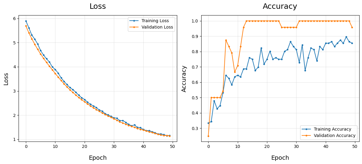
Plot Training History#
dw.plot_train_history() visualizes the training history of a fitted Keras model or history dictionary.
This function creates a grid of subplots to display the training and validation metrics over the epochs. You can pass a fitted model, in which case the history will be extracted from it. Alternatively, you can pass the history dictionary itself. This function will automatically detect the metrics present in the history and plot them all, unless a specific list of metrics is provided. The loss is plotted by default, but can be excluded by setting plot_loss to False.
Use this function to quickly analyze the model’s performance during training and identify potential issues such as overfitting or underfitting.
[161]:
# Create a sample classification dataset
X, y = make_classification(n_samples=1000, n_features=10, random_state=42)
X_train, X_test, y_train, y_test = train_test_split(X, y, test_size=0.2, random_state=42)
[162]:
# Create a simple example model
model = Sequential([
Input(shape=(10,)),
Dense(50, activation='relu'),
Dense(1, activation='sigmoid')
])
model.compile(optimizer='adam', loss='binary_crossentropy',
metrics=['accuracy', 'precision', 'recall'])
[163]:
# Fit the model
model.fit(X_train, y_train, epochs=20, batch_size=32, validation_split=0.2)
Epoch 1/20
20/20 ━━━━━━━━━━━━━━━━━━━━ 2s 27ms/step - accuracy: 0.4649 - loss: 0.7745 - precision: 0.4547 - recall: 0.4817 - val_accuracy: 0.5938 - val_loss: 0.6547 - val_precision: 0.5542 - val_recall: 0.6216
Epoch 2/20
20/20 ━━━━━━━━━━━━━━━━━━━━ 0s 3ms/step - accuracy: 0.6490 - loss: 0.6451 - precision: 0.6329 - recall: 0.6617 - val_accuracy: 0.7688 - val_loss: 0.5623 - val_precision: 0.7284 - val_recall: 0.7973
Epoch 3/20
20/20 ━━━━━━━━━━━━━━━━━━━━ 0s 3ms/step - accuracy: 0.7723 - loss: 0.5529 - precision: 0.7710 - recall: 0.7571 - val_accuracy: 0.8500 - val_loss: 0.5001 - val_precision: 0.8289 - val_recall: 0.8514
Epoch 4/20
20/20 ━━━━━━━━━━━━━━━━━━━━ 0s 4ms/step - accuracy: 0.8266 - loss: 0.4870 - precision: 0.8244 - recall: 0.8162 - val_accuracy: 0.8687 - val_loss: 0.4574 - val_precision: 0.8630 - val_recall: 0.8514
Epoch 5/20
20/20 ━━━━━━━━━━━━━━━━━━━━ 0s 4ms/step - accuracy: 0.8539 - loss: 0.4388 - precision: 0.8552 - recall: 0.8399 - val_accuracy: 0.8750 - val_loss: 0.4271 - val_precision: 0.8649 - val_recall: 0.8649
Epoch 6/20
20/20 ━━━━━━━━━━━━━━━━━━━━ 0s 3ms/step - accuracy: 0.8618 - loss: 0.4025 - precision: 0.8672 - recall: 0.8433 - val_accuracy: 0.8687 - val_loss: 0.4056 - val_precision: 0.8630 - val_recall: 0.8514
Epoch 7/20
20/20 ━━━━━━━━━━━━━━━━━━━━ 0s 3ms/step - accuracy: 0.8692 - loss: 0.3749 - precision: 0.8754 - recall: 0.8504 - val_accuracy: 0.8750 - val_loss: 0.3904 - val_precision: 0.8649 - val_recall: 0.8649
Epoch 8/20
20/20 ━━━━━━━━━━━━━━━━━━━━ 0s 4ms/step - accuracy: 0.8765 - loss: 0.3541 - precision: 0.8883 - recall: 0.8507 - val_accuracy: 0.8750 - val_loss: 0.3797 - val_precision: 0.8649 - val_recall: 0.8649
Epoch 9/20
20/20 ━━━━━━━━━━━━━━━━━━━━ 0s 4ms/step - accuracy: 0.8806 - loss: 0.3383 - precision: 0.8928 - recall: 0.8550 - val_accuracy: 0.8687 - val_loss: 0.3725 - val_precision: 0.8630 - val_recall: 0.8514
Epoch 10/20
20/20 ━━━━━━━━━━━━━━━━━━━━ 0s 4ms/step - accuracy: 0.8806 - loss: 0.3263 - precision: 0.8928 - recall: 0.8550 - val_accuracy: 0.8687 - val_loss: 0.3677 - val_precision: 0.8630 - val_recall: 0.8514
Epoch 11/20
20/20 ━━━━━━━━━━━━━━━━━━━━ 0s 4ms/step - accuracy: 0.8786 - loss: 0.3172 - precision: 0.8888 - recall: 0.8550 - val_accuracy: 0.8687 - val_loss: 0.3646 - val_precision: 0.8630 - val_recall: 0.8514
Epoch 12/20
20/20 ━━━━━━━━━━━━━━━━━━━━ 0s 3ms/step - accuracy: 0.8846 - loss: 0.3103 - precision: 0.8902 - recall: 0.8674 - val_accuracy: 0.8750 - val_loss: 0.3626 - val_precision: 0.8750 - val_recall: 0.8514
Epoch 13/20
20/20 ━━━━━━━━━━━━━━━━━━━━ 0s 3ms/step - accuracy: 0.8846 - loss: 0.3049 - precision: 0.8902 - recall: 0.8674 - val_accuracy: 0.8687 - val_loss: 0.3614 - val_precision: 0.8630 - val_recall: 0.8514
Epoch 14/20
20/20 ━━━━━━━━━━━━━━━━━━━━ 0s 4ms/step - accuracy: 0.8846 - loss: 0.3006 - precision: 0.8902 - recall: 0.8674 - val_accuracy: 0.8625 - val_loss: 0.3607 - val_precision: 0.8514 - val_recall: 0.8514
Epoch 15/20
20/20 ━━━━━━━━━━━━━━━━━━━━ 0s 3ms/step - accuracy: 0.8825 - loss: 0.2970 - precision: 0.8897 - recall: 0.8631 - val_accuracy: 0.8625 - val_loss: 0.3603 - val_precision: 0.8514 - val_recall: 0.8514
Epoch 16/20
20/20 ━━━━━━━━━━━━━━━━━━━━ 0s 3ms/step - accuracy: 0.8846 - loss: 0.2941 - precision: 0.8902 - recall: 0.8674 - val_accuracy: 0.8625 - val_loss: 0.3602 - val_precision: 0.8514 - val_recall: 0.8514
Epoch 17/20
20/20 ━━━━━━━━━━━━━━━━━━━━ 0s 3ms/step - accuracy: 0.8851 - loss: 0.2918 - precision: 0.8888 - recall: 0.8703 - val_accuracy: 0.8625 - val_loss: 0.3602 - val_precision: 0.8514 - val_recall: 0.8514
Epoch 18/20
20/20 ━━━━━━━━━━━━━━━━━━━━ 0s 3ms/step - accuracy: 0.8830 - loss: 0.2897 - precision: 0.8883 - recall: 0.8660 - val_accuracy: 0.8625 - val_loss: 0.3603 - val_precision: 0.8514 - val_recall: 0.8514
Epoch 19/20
20/20 ━━━━━━━━━━━━━━━━━━━━ 0s 3ms/step - accuracy: 0.8878 - loss: 0.2879 - precision: 0.8895 - recall: 0.8759 - val_accuracy: 0.8625 - val_loss: 0.3603 - val_precision: 0.8514 - val_recall: 0.8514
Epoch 20/20
20/20 ━━━━━━━━━━━━━━━━━━━━ 0s 3ms/step - accuracy: 0.8898 - loss: 0.2862 - precision: 0.8900 - recall: 0.8802 - val_accuracy: 0.8625 - val_loss: 0.3603 - val_precision: 0.8514 - val_recall: 0.8514
[163]:
<keras.src.callbacks.history.History at 0x7fe808b6d220>
[164]:
# Capture the history
history = model.history.history
[165]:
# Plot all metrics in the training history from a model
dw.plot_train_history(model)
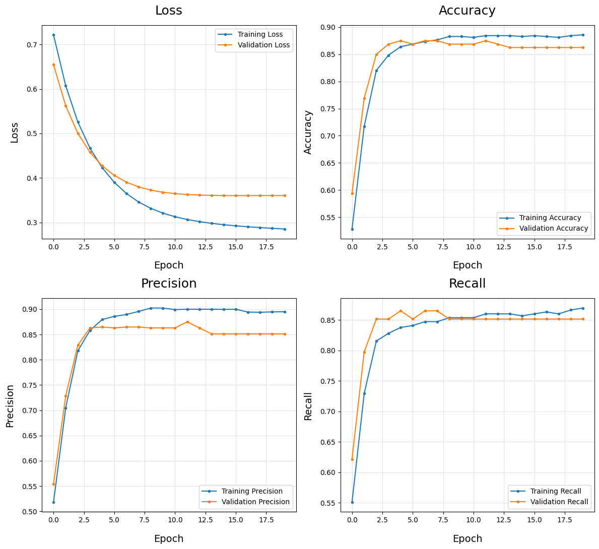
[166]:
# Plot the training history with specific metrics:
dw.plot_train_history(model, metrics=['accuracy', 'precision'])
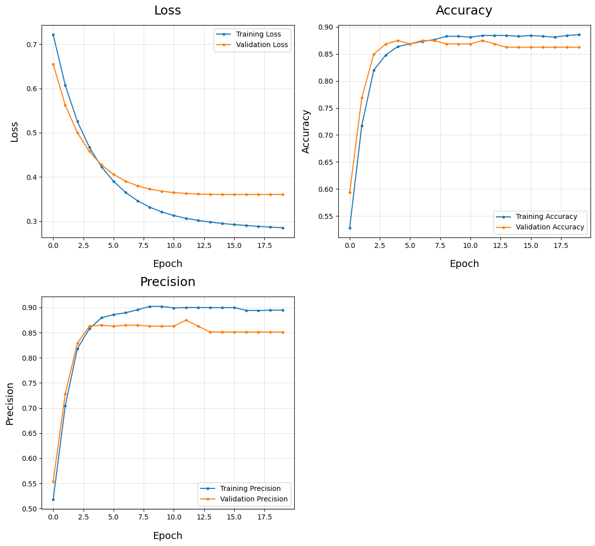
[167]:
# Plot the training history without the loss
dw.plot_train_history(model, plot_loss=False)
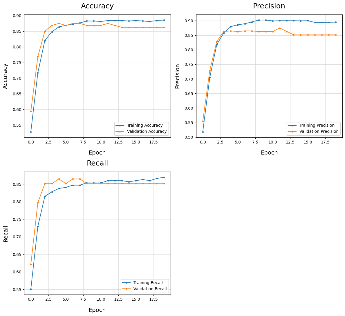
[168]:
# Create a another example model
model = Sequential([
Input(shape=(10,)),
Dense(50, activation='relu'),
Dense(1, activation='sigmoid')
])
model.compile(optimizer='adam', loss='binary_crossentropy',
metrics=['accuracy', 'precision', 'recall'])
[169]:
# Fit a model without specifying validation
model.fit(X_train, y_train, epochs=20, batch_size=32)
Epoch 1/20
25/25 ━━━━━━━━━━━━━━━━━━━━ 1s 1ms/step - accuracy: 0.5177 - loss: 0.7998 - precision: 0.2197 - recall: 0.0046
Epoch 2/20
25/25 ━━━━━━━━━━━━━━━━━━━━ 0s 2ms/step - accuracy: 0.5973 - loss: 0.6481 - precision: 0.9273 - recall: 0.1659
Epoch 3/20
25/25 ━━━━━━━━━━━━━━━━━━━━ 0s 1ms/step - accuracy: 0.7325 - loss: 0.5456 - precision: 0.8916 - recall: 0.4907
Epoch 4/20
25/25 ━━━━━━━━━━━━━━━━━━━━ 0s 1ms/step - accuracy: 0.8453 - loss: 0.4716 - precision: 0.9095 - recall: 0.7479
Epoch 5/20
25/25 ━━━━━━━━━━━━━━━━━━━━ 0s 1ms/step - accuracy: 0.8611 - loss: 0.4171 - precision: 0.8964 - recall: 0.7975
Epoch 6/20
25/25 ━━━━━━━━━━━━━━━━━━━━ 0s 1ms/step - accuracy: 0.8779 - loss: 0.3775 - precision: 0.8985 - recall: 0.8344
Epoch 7/20
25/25 ━━━━━━━━━━━━━━━━━━━━ 0s 1ms/step - accuracy: 0.8825 - loss: 0.3491 - precision: 0.8897 - recall: 0.8544
Epoch 8/20
25/25 ━━━━━━━━━━━━━━━━━━━━ 0s 1ms/step - accuracy: 0.8892 - loss: 0.3290 - precision: 0.8866 - recall: 0.8737
Epoch 9/20
25/25 ━━━━━━━━━━━━━━━━━━━━ 0s 1ms/step - accuracy: 0.8875 - loss: 0.3148 - precision: 0.8822 - recall: 0.8751
Epoch 10/20
25/25 ━━━━━━━━━━━━━━━━━━━━ 0s 1ms/step - accuracy: 0.8899 - loss: 0.3045 - precision: 0.8789 - recall: 0.8851
Epoch 11/20
25/25 ━━━━━━━━━━━━━━━━━━━━ 0s 1ms/step - accuracy: 0.8892 - loss: 0.2970 - precision: 0.8767 - recall: 0.8864
Epoch 12/20
25/25 ━━━━━━━━━━━━━━━━━━━━ 0s 1ms/step - accuracy: 0.8884 - loss: 0.2913 - precision: 0.8754 - recall: 0.8864
Epoch 13/20
25/25 ━━━━━━━━━━━━━━━━━━━━ 0s 1ms/step - accuracy: 0.8879 - loss: 0.2869 - precision: 0.8746 - recall: 0.8861
Epoch 14/20
25/25 ━━━━━━━━━━━━━━━━━━━━ 0s 2ms/step - accuracy: 0.8879 - loss: 0.2833 - precision: 0.8746 - recall: 0.8861
Epoch 15/20
25/25 ━━━━━━━━━━━━━━━━━━━━ 0s 1ms/step - accuracy: 0.8879 - loss: 0.2802 - precision: 0.8746 - recall: 0.8861
Epoch 16/20
25/25 ━━━━━━━━━━━━━━━━━━━━ 0s 2ms/step - accuracy: 0.8879 - loss: 0.2776 - precision: 0.8746 - recall: 0.8861
Epoch 17/20
25/25 ━━━━━━━━━━━━━━━━━━━━ 0s 2ms/step - accuracy: 0.8879 - loss: 0.2753 - precision: 0.8746 - recall: 0.8861
Epoch 18/20
25/25 ━━━━━━━━━━━━━━━━━━━━ 0s 2ms/step - accuracy: 0.8878 - loss: 0.2732 - precision: 0.8745 - recall: 0.8861
Epoch 19/20
25/25 ━━━━━━━━━━━━━━━━━━━━ 0s 2ms/step - accuracy: 0.8878 - loss: 0.2713 - precision: 0.8745 - recall: 0.8861
Epoch 20/20
25/25 ━━━━━━━━━━━━━━━━━━━━ 0s 2ms/step - accuracy: 0.8878 - loss: 0.2695 - precision: 0.8745 - recall: 0.8861
[169]:
<keras.src.callbacks.history.History at 0x7fe809179f10>
[170]:
# Plot a model that doesn't have validation data
dw.plot_train_history(model)
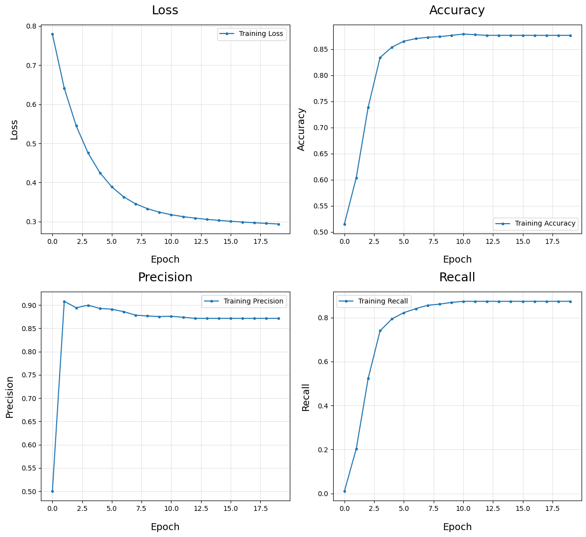
[171]:
# Plot the training history from a history dictionary
dw.plot_train_history(history=history)

Tools#
The dw.tools module provides helper tools used in data analysis, cleaning, and modeling. This module provides helper tools used in data analysis, cleaning, and modeling. It contains functions to check for duplicates in lists, split a dataframe into by numeric vs. categorical variables, and format numbers on the axis of a chart.
Log Transform - log_transform()
Check for Duplicates - check_for_duplicates()
Split Dataframe - split_dataframe()
Format Dataframe - format_df()
Format Chart Axis as Dollars - dollars()
Format Chart Axis as Thousands - thousands()
Calculate VIF - calc_vif()
Calculate PFI - calc_pfi()
Extract Coefficients - extract_coef()
Log Transform#
dw.log_transform() applies a log transformation to specified columns in a DataFrame.
This function applies a log transformation (base e) to the specified columns of the input DataFrame. The log-transformed columns are appended to the DataFrame with the suffix ‘_log’. If a column contains a negative value, a log transformation is not possible. In this case, a warning message will be printed, and the function will continue and try to transform additional columns.
Use this function when you need to log-transform skewed columns in a DataFrame to approximate a more normal distribution for modeling.
[172]:
# Plot histograms of skewed variables, dimensioned by the target variable
dw.plot_charts(df, plot_type='cont', cont_cols=skew_columns, hue='y', multiple='stack')
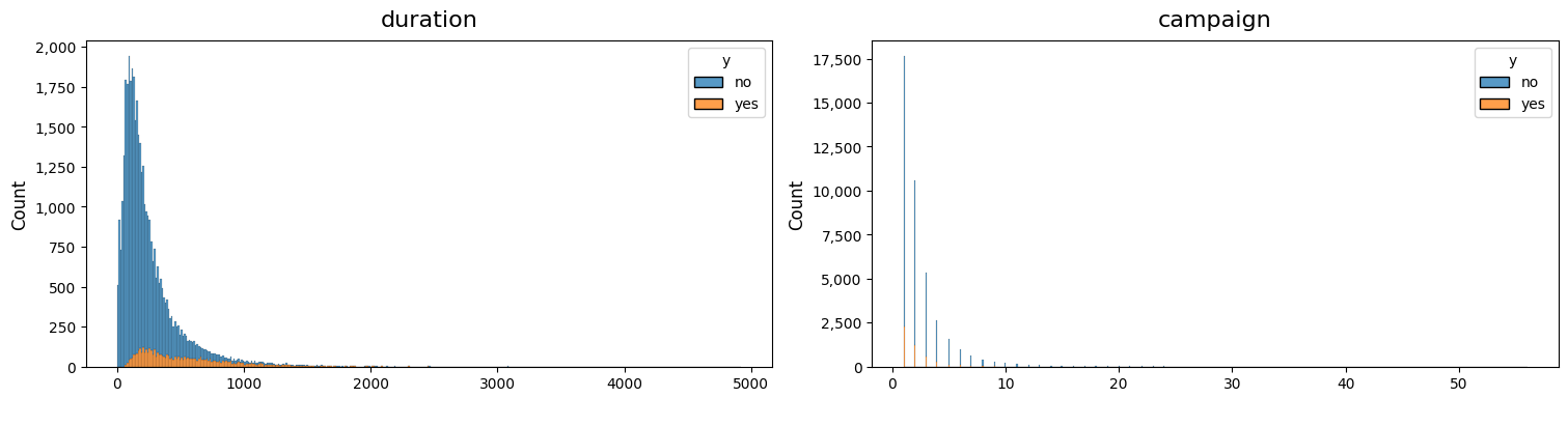
[173]:
# Specify columns that have a skewed shape
skew_columns = ['duration']
[174]:
# Log transform the specified columns in a dataframe
df_log = dw.log_transform(df, columns=skew_columns)
[175]:
# Notice the new column added with the _log suffix
df_log.info()
<class 'pandas.core.frame.DataFrame'>
RangeIndex: 41188 entries, 0 to 41187
Data columns (total 22 columns):
# Column Non-Null Count Dtype
--- ------ -------------- -----
0 age 41188 non-null float64
1 job 41188 non-null category
2 marital 41188 non-null category
3 education 41188 non-null category
4 default 41188 non-null category
5 housing 41188 non-null category
6 loan 41188 non-null category
7 contact 41188 non-null category
8 month 41188 non-null category
9 day_of_week 41188 non-null category
10 duration 41188 non-null float64
11 campaign 41188 non-null float64
12 pdays 41188 non-null float64
13 previous 41188 non-null float64
14 poutcome 41188 non-null category
15 emp.var.rate 41188 non-null float64
16 cons.price.idx 41188 non-null float64
17 cons.conf.idx 41188 non-null float64
18 euribor3m 41188 non-null float64
19 nr.employed 41188 non-null float64
20 y 41188 non-null category
21 duration_log 41188 non-null float64
dtypes: category(11), float64(11)
memory usage: 3.9 MB
[176]:
# Plot histograms of the log transformed variables, dimensioned by the target variable
dw.plot_charts(df_log, plot_type='cont', cont_cols=['duration_log'], hue='y', multiple='stack')
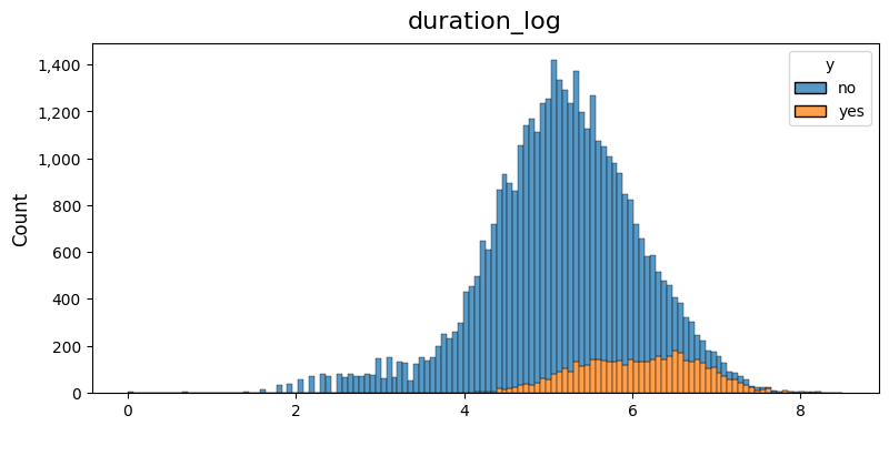
Note: You can also get this chart by just specifying the log_scale=True parameter in dw.plot_charts. But that does not save the log transformed data. So you have two options. If you want to transform the data for modeling, you would need to use dw.log_transform. But if you just want to evaluate if a log transformation would approximate a normal distribution, you can use dw.plot_charts with the log_scale=True parameter.
[177]:
# Example plot showing dw.plot_charts with log_scale=True
dw.plot_charts(df, plot_type='cont', cont_cols=skew_columns, hue='y', multiple='stack', log_scale=True)
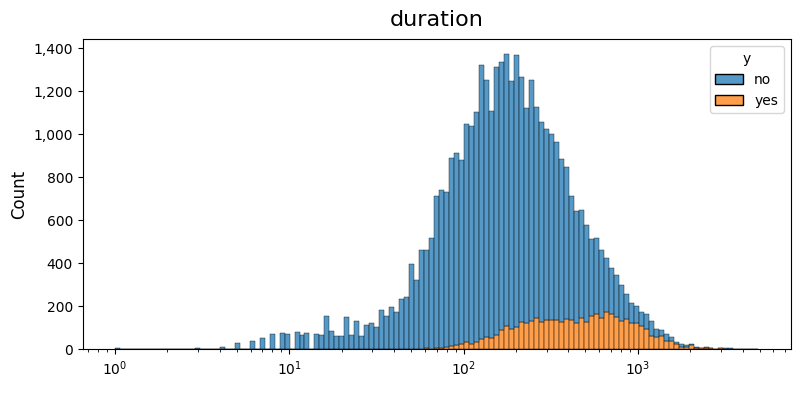
Check for Duplicates#
dw.check_for_duplicates() checks for duplicate items (ex: column names) across multiple lists.
This function takes an arbitrary number of lists and checks for duplicate items across the lists, as well as items appearing more than once within each list. It prints a summary of the items and the lists they appear in. Additionally, if a DataFrame is provided, it checks for any columns in the DataFrame that are missing from the lists and prints them.
Use this function when you are organizing columns in a large DataFrame into lists that represent their variable type (ex: num_columns, cat_columns). This helps to ensure you haven’t duplicated a column accidentally. And the optional DataFrame check helps you identify columns that haven’t been assigned to a list yet. This is really useful when you’re dealing with a large dataset.
[178]:
# Scan the data we have in the dataframe
df.head()
[178]:
| age | job | marital | education | default | housing | loan | contact | month | day_of_week | duration | campaign | pdays | previous | poutcome | emp.var.rate | cons.price.idx | cons.conf.idx | euribor3m | nr.employed | y | |
|---|---|---|---|---|---|---|---|---|---|---|---|---|---|---|---|---|---|---|---|---|---|
| 0 | 56.0 | housemaid | married | basic.4y | no | no | no | telephone | may | mon | 261.0 | 1.0 | 999.0 | 0.0 | nonexistent | 1.1 | 93.994 | -36.4 | 4.857 | 5191.0 | no |
| 1 | 57.0 | services | married | high.school | unknown | no | no | telephone | may | mon | 149.0 | 1.0 | 999.0 | 0.0 | nonexistent | 1.1 | 93.994 | -36.4 | 4.857 | 5191.0 | no |
| 2 | 37.0 | services | married | high.school | no | yes | no | telephone | may | mon | 226.0 | 1.0 | 999.0 | 0.0 | nonexistent | 1.1 | 93.994 | -36.4 | 4.857 | 5191.0 | no |
| 3 | 40.0 | admin. | married | basic.6y | no | no | no | telephone | may | mon | 151.0 | 1.0 | 999.0 | 0.0 | nonexistent | 1.1 | 93.994 | -36.4 | 4.857 | 5191.0 | no |
| 4 | 56.0 | services | married | high.school | no | no | yes | telephone | may | mon | 307.0 | 1.0 | 999.0 | 0.0 | nonexistent | 1.1 | 93.994 | -36.4 | 4.857 | 5191.0 | no |
[179]:
# Review the dtypes
df.info()
<class 'pandas.core.frame.DataFrame'>
RangeIndex: 41188 entries, 0 to 41187
Data columns (total 21 columns):
# Column Non-Null Count Dtype
--- ------ -------------- -----
0 age 41188 non-null float64
1 job 41188 non-null category
2 marital 41188 non-null category
3 education 41188 non-null category
4 default 41188 non-null category
5 housing 41188 non-null category
6 loan 41188 non-null category
7 contact 41188 non-null category
8 month 41188 non-null category
9 day_of_week 41188 non-null category
10 duration 41188 non-null float64
11 campaign 41188 non-null float64
12 pdays 41188 non-null float64
13 previous 41188 non-null float64
14 poutcome 41188 non-null category
15 emp.var.rate 41188 non-null float64
16 cons.price.idx 41188 non-null float64
17 cons.conf.idx 41188 non-null float64
18 euribor3m 41188 non-null float64
19 nr.employed 41188 non-null float64
20 y 41188 non-null category
dtypes: category(11), float64(10)
memory usage: 3.6 MB
[180]:
# Review the number of unique values in each column
df.nunique()
[180]:
age 78
job 12
marital 4
education 8
default 3
housing 3
loan 3
contact 2
month 10
day_of_week 5
duration 1544
campaign 42
pdays 27
previous 8
poutcome 3
emp.var.rate 10
cons.price.idx 26
cons.conf.idx 26
euribor3m 316
nr.employed 11
y 2
dtype: int64
[181]:
# Create column lists based on what we've learned for various variable types
cat_columns = ['job', 'marital', 'education', 'default', 'housing', 'loan', 'contact', 'month', 'day_of_week', 'previous', 'poutcome', 'y', 'y']
num_columns = ['age', 'duration', 'pdays', 'previous', 'emp.var.rate', 'cons.price.idx', 'cons.conf.idx', 'euribor3m', 'nr.employed']
[182]:
# Check for duplicate column names in the lists, since they were created manually
dw.check_for_duplicates(cat_columns, num_columns)
Items appearing in more than one list, or more than once per list:
previous (2): cat_columns, num_columns
y (2): cat_columns, cat_columns
[183]:
# Fix the duplicates
cat_columns = ['job', 'marital', 'education', 'default', 'housing', 'loan', 'contact', 'month', 'day_of_week', 'poutcome', 'y']
[184]:
# Re-check duplicates, and also see if we missed any columns in the dataframe
dw.check_for_duplicates(cat_columns, num_columns, df=df)
Items appearing in more than one list, or more than once per list:
None.
Columns in the dataframe missing from the lists:
campaign
[185]:
# Add the missing column to a list
num_columns.append('campaign')
[186]:
# Final re-check
dw.check_for_duplicates(cat_columns, num_columns, df=df)
Items appearing in more than one list, or more than once per list:
None.
Columns in the dataframe missing from the lists:
None.
Split Dataframe#
dw.split_dataframe() splits a DataFrame into categorical and numerical columns.
This function splits the input DataFrame into two separate DataFrames based on the number of unique values in each column. Columns with n or fewer unique values are considered categorical and are placed in df_cat, while columns with more than n unique values are considered numerical and are placed in df_num.
Use this function when you need to separate categorical and numerical columns in a DataFrame for further analysis or processing.
[187]:
# Split a dataframe in two, with unique values of 12 or less going into df_cat, the rest going into df_num
df_cat, df_num = dw.split_dataframe(df, n=12)
[188]:
# Review the categorical dataframe, which we can see is not a perfect split
df_cat.head()
[188]:
| job | marital | education | default | housing | loan | contact | month | day_of_week | previous | poutcome | emp.var.rate | nr.employed | y | |
|---|---|---|---|---|---|---|---|---|---|---|---|---|---|---|
| 0 | housemaid | married | basic.4y | no | no | no | telephone | may | mon | 0.0 | nonexistent | 1.1 | 5191.0 | no |
| 1 | services | married | high.school | unknown | no | no | telephone | may | mon | 0.0 | nonexistent | 1.1 | 5191.0 | no |
| 2 | services | married | high.school | no | yes | no | telephone | may | mon | 0.0 | nonexistent | 1.1 | 5191.0 | no |
| 3 | admin. | married | basic.6y | no | no | no | telephone | may | mon | 0.0 | nonexistent | 1.1 | 5191.0 | no |
| 4 | services | married | high.school | no | no | yes | telephone | may | mon | 0.0 | nonexistent | 1.1 | 5191.0 | no |
[189]:
# Review the numeric dataframe
df_num.head()
[189]:
| age | duration | campaign | pdays | cons.price.idx | cons.conf.idx | euribor3m | |
|---|---|---|---|---|---|---|---|
| 0 | 56.0 | 261.0 | 1.0 | 999.0 | 93.994 | -36.4 | 4.857 |
| 1 | 57.0 | 149.0 | 1.0 | 999.0 | 93.994 | -36.4 | 4.857 |
| 2 | 37.0 | 226.0 | 1.0 | 999.0 | 93.994 | -36.4 | 4.857 |
| 3 | 40.0 | 151.0 | 1.0 | 999.0 | 93.994 | -36.4 | 4.857 |
| 4 | 56.0 | 307.0 | 1.0 | 999.0 | 93.994 | -36.4 | 4.857 |
Observation: Sometimes there’s not a clear line, based on the unique value counts, that can be used to separate the categorical vs. numeric features. In practice, I don’t often split the dataframe, but just create lists of columns and then pass df[num_columns] or df[cat_columns].
Format Dataframe#
dw.format_dataframe() formats columns of a DataFrame as either large or small numbers.
This function formats the specified columns in the input DataFrame. Large numbers are formatted with commas as thousands separators, and small numbers are formatted with a specified number of decimal places. Use decimal to define how many decimal places to display.
Use this function when you need to format specific columns in a DataFrame for better readability or presentation purposes.
[190]:
# Load a dataframe that has a mix of a large and small numbers
results_df = pd.read_csv('data/results_df.csv', index_col=0)
[191]:
# Preview the data, note the large numbers with scientific notation, and small numbers with long decimals
results_df.head()
[191]:
| Iteration | Train MSE | Test MSE | Train RMSE | Test RMSE | Train MAE | Test MAE | Train R^2 Score | Test R^2 Score | Pipeline | Note | Date | |
|---|---|---|---|---|---|---|---|---|---|---|---|---|
| 0 | 1 | 3.588930e+09 | 3.561885e+09 | 59907.682665 | 59681.527129 | 44454.606285 | 44197.778286 | 0.606782 | 0.616300 | Model: linreg | No outliers. Drop ocean_proximity. LinReg | Aug 07, 2023 02:38 AM PST |
| 1 | 2 | 3.449797e+09 | 3.409325e+09 | 58734.974249 | 58389.423619 | 43054.713459 | 42812.841927 | 0.622026 | 0.632734 | transformer_ohe -> Model: linreg | No outliers. OHE. LinReg | Aug 07, 2023 02:40 AM PST |
| 2 | 3 | 2.924153e+09 | 2.832674e+09 | 54075.438033 | 53222.870883 | 38868.694712 | 38094.346879 | 0.679617 | 0.694853 | Transformer: ohe_poly2 -> Model: linreg | No outliers. OHE. Poly 2. LinReg | Aug 07, 2023 02:42 AM PST |
| 3 | 4 | 2.645702e+09 | 2.821643e+09 | 51436.387928 | 53119.139273 | 36930.866995 | 37336.066047 | 0.710126 | 0.696042 | Transformer: ohe_poly3 -> Model: linreg | No outliers. OHE. Poly 3. LinReg | Aug 07, 2023 02:44 AM PST |
| 4 | 5 | 2.984159e+09 | 2.895566e+09 | 54627.455531 | 53810.461446 | 39389.146063 | 38716.775476 | 0.673043 | 0.688078 | Transformer: ord_poly2 -> Model: linreg | No outliers. Ordinal. Poly 2. LinReg | Aug 07, 2023 02:46 AM PST |
[192]:
# Create a formatted dataframe for better readability only - not for data analysis
formatted_df = dw.format_df(results_df,
large_num_cols=['Train MSE', 'Test MSE', 'Train RMSE', 'Test RMSE', 'Train MAE', 'Test MAE'],
small_num_cols=['Train R^2 Score', 'Test R^2 Score'])
[193]:
# Review the formatted dataframe, which is much easier to read
formatted_df.head()
[193]:
| Iteration | Train MSE | Test MSE | Train RMSE | Test RMSE | Train MAE | Test MAE | Train R^2 Score | Test R^2 Score | Pipeline | Note | Date | |
|---|---|---|---|---|---|---|---|---|---|---|---|---|
| 0 | 1 | 3,588,930,442 | 3,561,884,680 | 59,908 | 59,682 | 44,455 | 44,198 | 0.61 | 0.62 | Model: linreg | No outliers. Drop ocean_proximity. LinReg | Aug 07, 2023 02:38 AM PST |
| 1 | 2 | 3,449,797,200 | 3,409,324,791 | 58,735 | 58,389 | 43,055 | 42,813 | 0.62 | 0.63 | transformer_ohe -> Model: linreg | No outliers. OHE. LinReg | Aug 07, 2023 02:40 AM PST |
| 2 | 3 | 2,924,152,998 | 2,832,673,985 | 54,075 | 53,223 | 38,869 | 38,094 | 0.68 | 0.69 | Transformer: ohe_poly2 -> Model: linreg | No outliers. OHE. Poly 2. LinReg | Aug 07, 2023 02:42 AM PST |
| 3 | 4 | 2,645,702,003 | 2,821,642,957 | 51,436 | 53,119 | 36,931 | 37,336 | 0.71 | 0.70 | Transformer: ohe_poly3 -> Model: linreg | No outliers. OHE. Poly 3. LinReg | Aug 07, 2023 02:44 AM PST |
| 4 | 5 | 2,984,158,898 | 2,895,565,761 | 54,627 | 53,810 | 39,389 | 38,717 | 0.67 | 0.69 | Transformer: ord_poly2 -> Model: linreg | No outliers. Ordinal. Poly 2. LinReg | Aug 07, 2023 02:46 AM PST |
Format Chart Axis as Dollars#
dw.dollars() formats a number as currency with thousands separators on a matplotlib chart axis.
This function takes a numeric value x and formats it as a string with thousands separators and a dollar sign prefix. The pos parameter is required by the matplotlib library for tick formatting but is not used in this function.
Use this function when you need to display currency values in a more readable format, particularly in the context of matplotlib or seaborn plots.
[199]:
# Load some data with large numbers
df_housing = pd.read_csv('data/housing_no_outliers.csv', index_col=0)
[200]:
# Review the data, notice the float values don't have comma separators or dollar signs
df_housing.head()
[200]:
| longitude | latitude | housing_median_age | total_rooms | total_bedrooms | population | households | median_income | median_house_value | ocean_proximity | |
|---|---|---|---|---|---|---|---|---|---|---|
| 0 | -122.23 | 37.88 | 41.0 | 880.0 | 129.0 | 322.0 | 126.0 | 83252.0 | 452600.0 | NEAR BAY |
| 1 | -122.22 | 37.86 | 21.0 | 7099.0 | 1106.0 | 2401.0 | 1138.0 | 83014.0 | 358500.0 | NEAR BAY |
| 8 | -122.26 | 37.84 | 42.0 | 2555.0 | 665.0 | 1206.0 | 595.0 | 20804.0 | 226700.0 | NEAR BAY |
| 15 | -122.26 | 37.85 | 50.0 | 1120.0 | 283.0 | 697.0 | 264.0 | 21250.0 | 140000.0 | NEAR BAY |
| 18 | -122.26 | 37.84 | 50.0 | 2239.0 | 455.0 | 990.0 | 419.0 | 19911.0 | 158700.0 | NEAR BAY |
[201]:
# Plot a chart with thousand dollars formatting on the X and Y axis
plt.figure(figsize=(12, 6))
plt.title('Median Income vs. Median House Value by Ocean Proximity', fontsize=18, pad=15)
sns.scatterplot(data=df_housing, x='median_income', y='median_house_value', hue='ocean_proximity')
plt.xlabel('Median Income', fontsize=14, labelpad=10)
plt.ylabel('Median House Value', fontsize=14, labelpad=10)
plt.gca().xaxis.set_major_formatter(FuncFormatter(dw.dollars)) # Add thousand dollars formatting on X axis
plt.gca().yaxis.set_major_formatter(FuncFormatter(dw.dollars)) # Add thousand dollars formatting on Y axis
plt.show()

Format Chart Axis as Thousands#
dw.thousands() formats a number with thousands separators on a matplotlib chart axis.
This function takes a numeric value x and formats it as a string with thousands separators. The pos parameter is required by the matplotlib library for tick formatting but is not used in this function.
Use this function when you need to display large numbers in a more readable format, particularly in the context of matplotlib or seaborn plots.
[202]:
# Plot a chart with thousands separators on the X and Y axis
plt.figure(figsize=(12, 6))
plt.title('Total Rooms vs. Population by Ocean Proximity', fontsize=18, pad=15)
sns.scatterplot(data=df_housing, x='total_rooms', y='population', hue='ocean_proximity')
plt.xlabel('Total Rooms', fontsize=14, labelpad=10)
plt.ylabel('Population', fontsize=14, labelpad=10)
plt.gca().xaxis.set_major_formatter(FuncFormatter(dw.thousands)) # Add thousands separators on X axis
plt.gca().yaxis.set_major_formatter(FuncFormatter(dw.thousands)) # Add thousands separators on Y axis
plt.show()
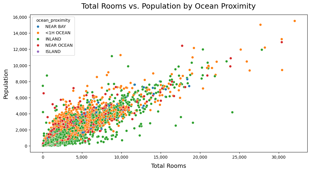
Calculate VIF#
dw.calc_vif() calculates the Variance Inflation Factor (VIF) for each feature in a dataset.
This function calculates the VIF for each feature in the input dataset. VIF is a measure of multicollinearity, which indicates the degree to which a feature can be explained by other features in the dataset. A higher VIF value suggests higher multicollinearity, and a VIF value exceeding 5 or 10 is often regarded as indicating severe multicollinearity.
By default, VIF will be calculated for all numeric columns in the X DataFrame. You can optionally specify columns with num_columns. You can also control how many decimal places are shown with decimal.
Use this function to identify features with high multicollinearity in your dataset before performing further analysis or modeling.
[203]:
# Calculate VIF for the numerical features in X
vif_df = dw.calc_vif(df)
[204]:
# Review the results
vif_df
[204]:
| Features | VIF | Multicollinearity | |
|---|---|---|---|
| 8 | euribor3m | 64.35 | High |
| 5 | emp.var.rate | 33.07 | High |
| 9 | nr.employed | 31.68 | High |
| 6 | cons.price.idx | 6.34 | Moderate |
| 7 | cons.conf.idx | 2.65 | Low |
| 4 | previous | 1.80 | Low |
| 3 | pdays | 1.61 | Low |
| 2 | campaign | 1.04 | Low |
| 0 | age | 1.02 | Low |
| 1 | duration | 1.01 | Low |
Calculate PFI#
dw.calc_pfi() calculates Permutation Feature Importance for a trained model.
This function calculates the Permutation Feature Importance (PFI) for each feature in the input dataset using a trained model. PFI measures the importance of each feature by permuting its values and observing the impact on the model’s performance. Features with higher permutation importance scores are considered more important for the model’s predictions.
The function returns a DataFrame with the feature names, mean permutation importance scores, and standard deviations of the scores. The DataFrame is sorted in descending order based on the mean scores. It’s just a wrapper around the Scikit-learn permutation_importance function to display the results in a convenient format.
Use this function to identify the most important features for a trained model and gain insights into the model’s behavior.
[205]:
# Prepare an X, y dataset
X = df[num_columns]
y = df['y']
[206]:
# Create and fit a Random Forest Classifier model
model = RandomForestClassifier(random_state=42)
model.fit(X, y)
[206]:
RandomForestClassifier(random_state=42)In a Jupyter environment, please rerun this cell to show the HTML representation or trust the notebook.
On GitHub, the HTML representation is unable to render, please try loading this page with nbviewer.org.
RandomForestClassifier(random_state=42)
[207]:
# Calculate Permutation Feature Importance
pfi_df = dw.calc_pfi(model, X, y, n_repeats=3, decimal=4)
[208]:
# Review the results
pfi_df
[208]:
| Feature | Importance Mean | Importance Std | |
|---|---|---|---|
| 1 | duration | 0.1289 | 0.0011 |
| 7 | euribor3m | 0.0763 | 0.0004 |
| 0 | age | 0.0501 | 0.0004 |
| 9 | campaign | 0.0313 | 0.0008 |
| 8 | nr.employed | 0.0200 | 0.0002 |
| 2 | pdays | 0.0169 | 0.0002 |
| 6 | cons.conf.idx | 0.0138 | 0.0002 |
| 5 | cons.price.idx | 0.0133 | 0.0003 |
| 3 | previous | 0.0119 | 0.0002 |
| 4 | emp.var.rate | 0.0083 | 0.0002 |
Extract Coefficients#
dw.extract_coef() extracts feature names and coefficients from a trained model.
This function traverses through the steps of a GridSearchCV or Pipeline object and extracts the feature names and coefficients from the final trained model. It attempts to handle transformations such as ColumnTransformer and feature scaling steps. However, due to the complexity of some transformations, and inconsistent support on tracking feature names, the final output feature names may be different than the input.
Note: This function currently supports only single target regression problems. It also checks against a list of known classes that support coefficient extraction. This list may not be comprehensive.
[209]:
# Create some column lists we can use to target the right kind of variables
all_housing = list(df_housing.columns)
num_housing = [col for col in all_housing if df_housing[col].dtype in ['int64', 'float64']]
cat_housing = [col for col in all_housing if df_housing[col].dtype in ['object', 'category', 'string']]
[210]:
# Prepare an X, y dataset
X = df_housing[num_housing].drop(columns='median_house_value')
y = df_housing['median_house_value']
[211]:
# Create a pipeline
pipe = Pipeline([
('scaler', StandardScaler()),
('model', Ridge())
])
[212]:
# Fit the pipeline
pipe.fit(X, y)
[212]:
Pipeline(steps=[('scaler', StandardScaler()), ('model', Ridge())])In a Jupyter environment, please rerun this cell to show the HTML representation or trust the notebook. On GitHub, the HTML representation is unable to render, please try loading this page with nbviewer.org.
Pipeline(steps=[('scaler', StandardScaler()), ('model', Ridge())])StandardScaler()
Ridge()
[213]:
# Extract the feature names and coefficients
dw.extract_coef(pipe, X,)
[213]:
| Feature | Coefficient | |
|---|---|---|
| 0 | longitude | -76,016.12 |
| 1 | latitude | -82,155.60 |
| 2 | housing_median_age | 8,727.70 |
| 3 | total_rooms | -19,698.35 |
| 4 | total_bedrooms | 38,903.99 |
| 5 | population | -38,304.18 |
| 6 | households | 22,984.43 |
| 7 | median_income | 61,808.67 |
[ ]: